Calculating Wedge Diagrams and Cost Curves

The Energy Policy Simulator (EPS) can break apart a policy package and illustrate the effects of each component policy within that package. The simulator produces two types of graphs of these policy-by-policy effects: wedge diagrams and cost curves. Both graph types are available for total GHG emissions, and wedge diagrams (but not cost curves) are also available for sector-specific GHG emissions and for avoided premature deaths.

To see examples of these graphs, and to learn how to read and understand them, see this location in the Tour of the Web Interface video.

Unlike most graphs, wedge diagrams and cost curves are only available in the web application, not in Vensim. This is because multiple model runs are required to calculate the data for one of these graphs. This documentation page explains the procedure the web application uses to produce these graphs.

Overview

Wedges vs. Cost Curve Boxes in This Documentation Page

For brevity and clarity, this documentation page discusses how wedge thicknesses are calculated. It does not mention cost curve boxes in every place where wedges are mentioned. All of the steps discussed for wedges also apply to cost curve box widths. Some details particular to cost curves appear at the end of this page.

Metric Used in This Documentation Page

As noted above, wedge diagrams are used to display several different metrics, such as total GHG emissions and avoided premature mortality. The calculation procedure to build the graph is the same in each case. Only different output variables are used. Therefore, the procedure explanation on this page refers to Total GHG Emissions for simplicity. The procedure is analogous for any other metric.

Policies and Policy Groups

Each policy that forms a single wedge is actually a set of a few different policy levers. Generally, all the subscripted elements of a given policy will be tested together. We call this a "policy group." For example, the policy "Building Energy Efficiency Standards" can be set to different values for different building types (urban residential, rural residential, or commercial) and different building components (heating, cooling, lighting, etc.). All of these settings are considered a single policy and will be tested together to form a single wedge for "Building Energy Efficiency Standards."

In rare cases, multiple policy levers (not just subscripted elements of a single lever) may be grouped as a single wedge. For example, the policies "Change Electricity Exports" and "Change Electricity Imports" are two separate policy levers, but they are grouped into a single wedge called "Electricity Imports and Exports."

The way in which policies are grouped is adjustable. In WebAppData.xlsx, on the "Policy Characteristics" tab, the "Policy Group" column specifies which policies should be grouped together into a single wedge and what that wedge should be called. Refer to that column for a complete list of all policies and wedge groupings.

Simplified Procedure

In EPS releases prior to 3.1.0, the wedge diagrams and cost curves used a straightforward calculation procedure. It is worthwhile to understand this simplified procedure, because the more refined procedure used in EPS 3.1.0 and later evolved from this simple procedure.

Simplified procedure steps:

• Run the scenario with all policies enabled and note the emissions level.

• Disable one policy and see how much emissions rise (relative to the scenario with all policies enabled). This is that policy's contribution to abatement.

• Re-enable the policy that was just disabled. Then disable the next policy and see how much emissions rise (relative to the scenario with all policies enabled).

• Repeat until all policies are tested.

• The resulting individual policy contributions will not sum to the total abatement from the policy package due to policy interactions. Therefore, we scale all of those wedges up or down by the same multiplier (say, 1.1 or 0.9) to make the wedges precisely fit the abatement of the package as a whole.

This procedure involves disabling one policy at a time in the context of the entire policy package. Therefore, it is useful for capturing policy interactions, portraying how important each individual policy is in the context of the rest of the policy package.

Flaws in the Simplified Procedure

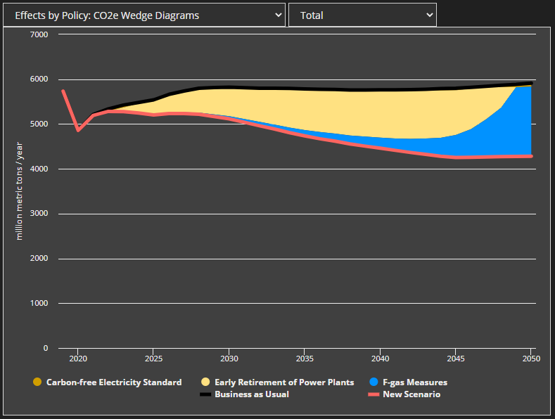
The simplified procedure works pretty well in most cases. However, one circumstance in which is performs poorly is if two policies have mostly overlapping effects (for instance, a clean electricity standard and accelerated retirement of fossil electricity plants). Both of these policies cause fossil plants to retire, and they get replaced by clean energy. If you disable one of them, the other one "picks up the slack," so emissions don't rise very much. The same thing happens if you disable the other one.

This can be a particular problem if there is a third, unrelated policy in the mix. That policy, which targets unrelated emissions, can tend to get all the credit for abatement. For example, if the third policy reduces F-gas process emissions in Industry, the entire thickness of the policy package can be erroneously ascribed to the F-gas reduction policy, because neither of the electricity sector policies is getting credit for the electricity sector reductions. Here is an example where the F-gas policy "takes over" in the latter years of the model run, when the two electricity sector policies are almost entirely overlapping.

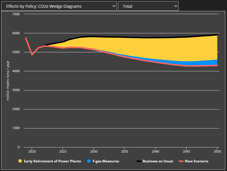
Here is the correct size of the F-gas wedge, which we see if we disable one of the two overlapping electricity sector policies, so the other one gets the credit for the electricity sector abatement:

It is possible to avoid these interactions by testing each policy individually. That is, in the policy package, you enable one policy at a time, checking to see how much emissions fall each time, to get the raw wedge thicknesses. Then you scale by a multiplier to make the wedges fit the total abatement of the package. The problem with this approach is that it fails to capture any policy interactions at all, which is important in many cases. Two examples are: (1) fuel shift to hydrogen in industry + shift hydrogen production to electrolysis, or (2) subsidize renewable energy + add flexibility to the grid, to accommodate more renewable energy. In each of these circumstances, testing the policies individually will fail to show the importance of the policies for decarbonization, because they rely on each other to deliver the large-scale abatement.

So, the goal is to limit the effects of interactions we don't want but keep interactions we do want. This turns out to be a trade-off, without a single correct "solution," but more of a compromise.

The best approach identified to date is to break each policy wedge into one wedge per sector (with sectors here corresponding to normal model sectors (transport, buildings, etc.) but breaking industry into energy-related emissions and process emissions). The policies' sectoral components are scaled to fit the total abatement of the policy package from that particular sector. Then, the sectors are scaled to fit the size of the overall abatement of the policy package. For example, this constrains the F-gas policy to only achieve the abatement derived from industrial process emissions, because the F-gas policy doesn't affect other sectors (at least, not perceptibly). This helps constrain policies from using the degree to which they affect one sector to influence their wedge sizes in other sectors. (Every policy can still affect multiple sectors, but each policy's sectoral component is the only thing that can influence that sector.)

This doesn't perfectly solve every case (you can still have two heavily-overlapping policies in the same sector do odd things, or cede credit to a third non-overlapping policy within that same sector), but it does catch and fix many of the problematic situations that can arise under the current methodology, without disabling any policy interactions.

Full Procedure

Here is a step-by-step description of the new and improved procedure. This example discusses wedge diagrams and mentions cost curves at the end.

Step 1

Obtain a list of all the component variables for the metric being graphed. In the case of CO₂e abatement, the components are emissions (or sequestration) from different sectors, which sum to the total net CO₂e emissions for the modeled region. The component variables will be listed in WebAppData.xlsx in the Vensim Names of Graphed Variables column, in the row for the relevant wedge diagram. The order in which the variables are listed does not matter. As of EPS 3.1.0, for the Total CO₂e Abatement wedge diagram, they should be:

• Output Total CO2e Emissions by Sector[transportation sector]
• Output Total CO2e Emissions by Sector[electricity sector]
• Output Total CO2e Emissions by Sector[district heat and hydrogen sector]
• Output Total CO2e Emissions by Sector[LULUCF sector]
• Output Total CO2e Emissions by Sector[geoengineering sector]
• Output Industry Sector Process Emissions in CO2e Excluding Ag and Waste
• Output Industry Sector Energy Related CO2e Emissions Excluding Ag and Waste
• Output Agriculture CO2e Emissions
• Output Waste Management CO2e Emissions
• Output Buildings Sector CO2e Emissions

Other wedge diagrams, such as the one for avoided premature mortality, may have fewer variables or just one variable listed in WebAppData.xlsx. The procedure here should work for all of these graphs. (If only one variable is listed, the procedure should produce results essentially identical to what we had in EPS 3.0.0 before the improved methodology was introduced.)

The directions in this post will refer to each variable listed above as a "sector," even though some of them (such as Industry Process Emissions and Industry Energy Related Emissions) are not technically sectors. They don't need to actually be sectors. The important thing is that the variables must sum to the metric you want graphed.

Step 2

We will assume you have a policy scenario, either created by the user in the web app, or defined by a .cin file and included as a reference scenario in the web app.

Just as in EPS 3.0.0 and earlier, certain policies are grouped, which means that they are treated as a single policy for purposes of drawing wedges. This has not changed. The groups are still defined in WebAppData.xlsx on the PolicyLevers tab in the Policy Group column. Generally, all the subscripted elements of a single lever are treated as part of the same group. (For example, a building component energy efficiency standard applied to heating systems and a building component energy efficiency standard applied to cooling systems are both going to be part of the building component energy efficiency standard policy group, and this group will have a single wedge.) In rare cases, different levers will be grouped. For example, the four different policies that target F-gas process emissions (F-gas substitution, F-gas destruction, F-gas recovery, F-gas eqpt. maintenance/retrofit) are assigned to the same F-gas Measures group, so they will be drawn as a single wedge. This prevents the fragmentation of the wedge diagram into many tiny wedges.

Any policy lever that has a blank entry in the Policy Group column is to be omitted from the wedge diagram entirely. This is also the same behavior has we have had in EPS 3.0 and prior. Currently, the only excluded levers are control settings, which are not policies, and which move the BAU case line along with the policy line, so they are not compatible with wedge diagrams or cost curves.

Step 3

Perform a series of model runs as follows:

• One run with all of the policies enabled (i.e. at the settings and with the implementation schedules set by the user, or the .cin file and FoPITY files for reference scenarios)

• One run with all of the policies disabled (set to BAU values, usually zero for policy levers)

• One run per policy group, with that policy group disabled, but all other policy groups in the scenario enabled

Any levers that do not have a Policy Group specified in WebAppData.xlsx (meaning they are to be omitted from the wedge diagram) should remain enabled throughout (even for the run that says "all of the policies disabled" in the bulleted list above), because it is likely a control setting and should always be affecting model output.

Remember the values produced for each of the component variables (listed in "Step 1" above) for each of these model runs.

Step 4

Calculate the unscaled wedge component sizes.

Each policy group can affect each of the component variables.

• For each policy group:
  • For each component variable:
    • For "reduction wedge" type charts, such as CO2e emissions abatement: Subtract the value from the model run with all policy groups enabled from the value from the model run with only this policy group disabled. This is the raw value attributable to this policy's contribution to this component variable. For example, if Output Total CO2e Emissions by Sector[transportation sector] is 30 with all policies enabled and is 35 with Policy Group 1 disabled, then Policy Group 1's contribution to the Output Total CO2e Emissions by Sector[transportation sector] component variable is (35 - 30) = 5.
    • For "increase wedge" type charts, such as avoided premature mortality: Take the inverse (negative) of the value above. For example, if avoided premature deaths is 60 with all policies enabled and 55 with this policy group disabled, the wedge thickness is 5, not -5.

In other words, when the policy group makes beneficial progress on the metric (which is a reduction in emissions, or an increase in avoided premature mortality), the wedge thickness should be positive. The wedge thickness should be negative if the policy group is harmful to the metric (increases emissions, or reduces avoided premature mortality). You can tell whether positive or negative changes are beneficial or harmful to the metric by checking whether the chart type is an "increase wedge" or "reduction wedge" in the Graph Style column of the OutputGraphs tab in WebAppData. Remember that we're testing each policy group by disabling it, not by enabling it, so if emissions rise when a policy group is disabled, this means the policy group was making a beneficial contribution to the metric. Similarly, if disabling a policy group causes avoided deaths to fall (i.e. more deaths), that means that policy group was making a beneficial contribution to that metric.

This is generally how raw wedge thicknesses were already calculated in EPS 3.0.0. The key difference as of 3.1 is that now we are doing this calculation separately for each component variable, rather than for a single metric variable taken as a whole. That is, we are adding the inner "For" loop, while the outer "For" loop and wedge thickness calculation should already exist.

Negative values were relatively uncommon under the old approach but will be much more common now, because it is common for a policy that is beneficial overall to have negative effects on at least one of the component variables. For instance, a policy might reduce emissions in the transportation sector by 100 units but increase energy-related emissions in the industrial sector by 2 units, so it will have a positive raw wedge thickness for the component variable Output Total CO2e Emissions by Sector[transportation sector] but a negative raw wedge thickness for the component variable Output Industry Sector Energy Related CO2e Emissions Excluding Ag and Waste.

Step 5

Replace all negative wedge thicknesses with zeroes. We can't have negative thicknesses on the graph, and including the negative numbers interferes with the scaling we need to perform.

Step 6

Calculate the thickness of each component variable (i.e. each sector).

For each component variable (i.e. each sector):

• Calculate the effect of the entire policy package (with all policies enabled) on this sector, by comparing the run with all policies enabled to the run with all policies disabled. This is done similarly to step 4, except you're comparing the case with all policies to the case with no policies, instead of disabling one particular policy group at a time. This is the total thickness of all policies' effects on this sector.

• If it is negative, change it to zero.

Step 7

Calculate scaling factors. Each component variable (i.e. each sector) gets one scaling factor. That scaling factor is used for all policy groups' effects on that sector. These are calculated the same way we currently calculate scaling factors, except that they are done on a sector-by-sector basis, instead of just once for the whole policy package.

For each sector:

• Sum up the raw thicknesses of all the policy groups' contributions to this sector, after removing zeroes (i.e. the output of "Step 5" above).

• Divide the sector's total thickness (as calculated in Step 6) by the sum of the policy groups' raw contributions to this sector, calculated immediately above.

This is that sector's scaling factor. Repeat for each sector.

Step 8

For each sector, multiply every policy group's contribution to that sector by that sector's scaling factor. All results should be zero or positive, because we removed negative values in step 5 (from the policy group contributions) and in step 6 (from the sector wedge sizes).

We now have sectorally-scaled wedges.

Step 9

We now restore values for policies whose beneficial effect is larger than the overall thickness of the sector. We need to do this because there may be a sector whose overall contribution to the metric is non-beneficial (or only mildly beneficial), but the policy makes a larger, beneficial contribution to that sector. A key example here is the combination of two policies: fuel switching to hydrogen and the hydrogen electrolysis policy. The fuel switching to hydrogen will cause emissions to increase in the hydrogen supply sector, because it increases demand for hydrogen relative to BAU. The hydrogen electrolysis policy can greatly lower or eliminate these emissions. If the hydrogen supply sector has a negative wedge thickness, since its emissions have increased relative to BAU, this would cause the hydrogen electrolysis policy effect to be scaled down to zero. This is wrong - it is simply that the hydrogen electrolysis policy is targeting emissions that didn't exist in the BAU case.

We can't just look for sectors where the overall contribution to the metric is non-beneficial, because this misses compensating effects. For example, if the fuel shift to hydrogen causes hydrogen supply sector emissions to increase by 800 units, and hydrogen electrolysis causes hydrogen supply sector emissions to decrease by 801 units, the final wedge thickness of the hydrogen supply sector will be 1. But it would be wrong to scale the hydrogen electrolysis policy down to size 1, to fit the sector's overall wedge size, because that policy is contributing 801 units of abatement.

We fix this by importing the values for policy groups' impacts on sectors from the raw wedge sizes (i.e. before we scaled) if that policy group has a beneficial impact larger than the size of the sector.

For each sector:

• Compare each policy group's raw contribution to that sector after removing negative values (the output of Step 5) to the overall size of that sector (the output of Step 6)
• If the policy group's contribution to that sector is larger than the sector's overall size, replace that policy group's thickness (as calculated in Step 8) with the unscaled thickness (as calculated in Step 5).

We should still have no negative values.

Step 10

We are done working in terms of sectors.

We now need to rescale all policy groups' effects on all sectors to match the total policy package size. Take the difference between the model run with all policies enabled and the run with no policies enabled, but summed across all sectors. (This can be calculated from the raw emissions data in Step 3, or the difference for each sector was already calculated in Step 6, prior to changing negative values to zero.) You should have just one number (in any given model year) that contains the total difference between the BAU line and the Policy Case line on the graph.

Sum the effects of all policy groups on all sectors, as calculated in the output of Step 9.

Divide the total package size by the sum of all policy groups' effects. This is the package scaling factor.

Multiply every policy group's effect on every sector (the output of Step 9) by the package scaling factor.

We now have final, scaled wedge components.

Step 11

Sum up the wedge components of each policy group (the output of Step 10) across all sectors. That way, each policy group ends up with just one wedge. For example, we sum the effects of the carbon tax across the industry sector, the transport sector, the buildings sector, etc.

Step 12

For an "increase wedge" diagram, such as avoided premature mortality, we are done. There is no step 12.

For a "reduction wedge" diagram, such as CO2e Emissions, we convert our final wedges into a wedge diagram by stacking them on top of a transparent wedge that represents the "remaining emissions." The remaining emissions are simply the emissions you got from the model run with all policies enabled (in Step 3), with no modifications.

Note that in any year where the policy case line is worse than BAU (i.e. has moved in the opposite direction from the metric, such as increased emissions or decreased avoided premature mortality), no wedges are shown in the gap between the policy case line and the BAU line. Wedges are only shown to color in the space between the policy case line and the BAU line when the policy case line is more beneficial than the BAU line for that metric.

Cost Curves

The abatement cost curve needs to know the average annual abatement of each policy group over the model run. Rather than calculating this itself, it should piggyback off the calculations done for the wedge diagram. That is, it should use the annual output from Step 11, sum across all model run years, and divide by the number of model run years. Once you have the width of each box, the Y-axis value for each box is calculated in the same way as before 3.1.0, using the new box width.

Closing Notes

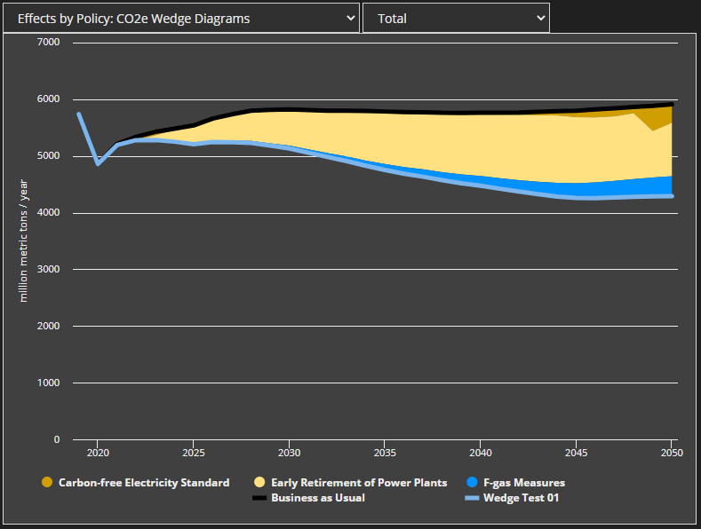
Here's what a scenario similar to the first graph in this post looks like using the new procedure. The blue line for F-gas Measures no longer takes over the whole policy package as the two electricity-sector policies become increasingly overlapping in later years.

The new procedure is designed to be backward-compatible with old EPS versions, so that the modern web app software can continue to build and deploy older models. To use the new procedure, you must list the component variables that make up the metric being graphed in the wedge diagram in WebAppData.xlsx, in the “OutputGraphs” tab, in the “Vensim Names of Graphed Variables” column. If you do not do this, the web app will still build and run without errors, but you will get wedge and cost curve results based on the old procedure. The component variables that make up a given metric will not vary by model region, so this should be a simple copy-and-paste operation.

The cost curves now only need one variable specified instead of two, as they rely on widths calculated for the wedge diagram.

---

This page was last updated in version 3.5.0.