Architectural Design
The Energy Policy Simulator (EPS) is a System Dynamics model that assesses the effects of numerous energy and environmental policies on a variety of metrics, including the emissions of 12 pollutants; cash flow changes for government, industry, and consumers; the composition of the electricity generation fleet; the usage of various fuels; lives saved from reduced particulate emissions; and more. The model is designed to operate at national scale, but versions for states/provinces and cities have also been created. It includes five major sectors: transportation, electricity supply, buildings, industry (including agriculture), and land use/forestry, each of which contains many variables and a variety of policies. It also has a number of other components that cover additional emissions sources or sinks, or which give the model additional capabilities. These include district heating, carbon capture and sequestration, research and development, fuels, hydrogen supply, geoengineering, and a variety of useful output metrics. The model reports outputs at annual intervals. A customizable policy implementation schedule allows for policies to be phased in with any given level of stringency in any particular year, as desired by the user.
Unlike many energy and economic computer models, the EPS does not construct a future business-as-usual (BAU) or reference scenario. Instead, it uses a BAU scenario (based on the results of other scientists' studies and models) as input data. The EPS then modifies the BAU scenario in response to the policy settings selected by the user. This approach enables us to take advantage of the good work that has been done in this field while providing novel capabilities to analyze policy options that are immediately useful to policymakers and suggest specific policy actions that could be undertaken. (The electricity and transportation sectors are exceptions. Policies in the electricity sector can affect decisions about which types of power plants to build and how plants are dispatched, so a decision-making framework must be employed. The decisions made by this framework using BAU input data may result in outputs that are different from those of other models, so in order to ensure our policy case is identical to our BAU case when all of the policies are disabled, we need to run BAU input data through our decision-making logic to construct a BAU case. Similar reasoning applies to technology selection and use in the transportation sector.)
System Dynamics
There exist a variety of approaches to representing the economy and the energy system in a computer simulation. The EPS is based on a theoretical framework called System Dynamics. As the name suggests, this approach views the processes of energy use and the economy as an open, ever-changing, non-equilibrium system. This may be contrasted with approaches such as computable general equilibrium (CGE) models, which regard the economy as an equilibrium system subject to exogenous shocks, or disaggregated technology-based models, which focus on the potential efficiency gains or emissions reductions that could be achieved by upgrading specific types of equipment.
System Dynamics models often include "stocks," or variables whose value is remembered from timestep to timestep, and which are affected by "flows" into and out of these variables. The EPS uses stocks for two purposes: tracking quantities that grow or shrink over time (such as the total solar electricity generation capacity) and tracking differences from the BAU input data that tend to grow over the course of the model run (for instance, the cumulative differences in the potential fuel consumption of the light-duty vehicle fleet caused by enabled policies).
System Dynamics models often use the output of the previous timestep's calculations as input for the following timestep. The EPS follows this convention, with quantities such as the electricity generation fleet, the types and efficiencies of building components, etc. remembered from one year to the next. Therefore, an efficiency improvement in an early year will result in fuel savings in all subsequent years, until the improved vehicle/building component/etc. is retired from service. The Industry sector is handled differently: since the available input data come in the form of potential reductions in fuel use and process-related emissions for each policy, we gradually implement these reductions (with corresponding implementation costs), rather than recursively tracking a fleet-wide efficiency. (Due to the diverse forms that input data take in the sectors we model, rarely does one calculation approach work for all sectors. Accordingly, the EPS attempts to use whichever approach makes the most sense in the context of each specific sector.)
Subscripts (Arrays)
The model's structure can be thought of as occurring along two dimensions: visible structure that pertains to the equations that define relationships between variables (viewable as a flowchart in Vensim) and behind-the-scenes structure that consists of arrays and their elements, which contain data and are acted on by the equations. For example, the transportation sector's visible structure consists of policies (such as a fuel economy standard), input data (such as the BAU cargo distance traveled- that is, passenger-miles or freight ton-miles), and calculated values, such as the quantities of fuels used by the vehicle fleet. The arrays in the behind-the-scenes structure of the transportation sector consist of vehicle categories (light-duty vehicles (LDVs), heavy-duty vehicles (HDVs), aircraft, rail, ships, and motorbikes), cargo types (passengers or freight), and fuel types (petroleum gasoline, petroleum diesel, electricity, etc.). The model generally will perform a separate set of calculations, based on a separate set of input data, for every combination of array elements. For example, the model will calculate different fuel economies for passenger HDVs, freight HDVs, passenger aircraft, freight aircraft, and so forth.
In Vensim, an array variable is called a "subscripted variable," a single dimension of an array is called a "subscript," and the possible values an array dimension may take are called "subscript elements." For example, the variable called "Fleet Avg Fuel Economy[vehicle type, cargo type, vehicle technology]" is a subscripted variable, "vehicle type," "cargo type," and "vehicle technology" are all subscripts, and the "vehicle type" subscript has the elements "LDVs," "HDVs," "aircraft," "rail," "ships," and "motorbikes." Almost every variable in the EPS is subscripted.
Calculation Flow
The following diagram shows the major pieces of the model, and the arrows denote the order of calculation, not the flow of energy. For example, the amount of electricity required is calculated in the sectors that can consume electricity (Industry, Buildings, Transportation, District Heat, Hydrogen Supply, Geoengineering), and then this result is fed into the Electricity Sector, which determines how to generate the necessary quantity of electricity.
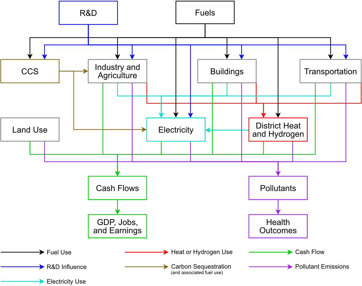
The model's calculation logic begins with the fuels sheet, where basic properties of all fuels are set and policies that affect the price of fuels are applied. Information about the fuels is used in the three "demand sectors": transportation, buildings, and industry (including agriculture). These sectors calculate their own emissions from direct fuel use- e.g. fossil fuels burned in vehicles, buildings, and industrial facilities. These sectors also specify a quantity of electricity, heat, and/or hydrogen (energy carriers supplied by other parts of the model) required in each year. The electricity, district heat, and hydrogen supply sectors consume fuel to supply the energy needs of the three demand sectors. The model also has a land use, land use change, and forestry (LULUCF) sector, which handles the emissions of pollutants and the sequestration of CO2 from existing forests, afforestation/reforestation, deforestation and timber harvesting, etc. All of these sectors produce emissions of each pollutant, which are summed on the Cross-Sector Totals sheet. Then, on the Additional Outputs sheet, these changes in pollutant emissions are then multiplied by health incident-per-ton multipliers derived from gridded air quality models and concentration-response functions to obtain health outcomes.
Like pollutants, cash flow impacts are summed from various sectors on the Cross-Sector Totals sheet. Cash flows are calculated separately for particular actors (government, non-energy industries, labor and consumers, and various energy-supplying industries), with impacts on non-energy industries further divided up among various ISIC codes (parts of the economy). Calculation of changes in spending (for example, on capital equipment, fuel, and O&M) is also carried out at this stage, on the Cost Outputs sheet. All of the direct financial results are then fed into the EPS's input-output (I/O) model to obtain GDP, jobs, and employee compensation impacts. There is also a feedback loop from the I/O model to the three demand sectors (not shown on the diagram), so the energy use and emissions associated with induced and indirect economic activity are captured (see the Macroeconomic Feedbacks sheet).
There are two model components that affect the operation of various sectors. A set of R&D levers allows the user to specify improvements in fuel economy and decreases in capital cost for technologies in the sectors (except LULUCF) and in the carbon capture and sequestration (CCS) module. These improvements are additional to improvements in the BAU case, and additional to any improvements calculated by the endogenous learning mechanism in response to policies that boost technology deployment. The CCS module alters the Industry and Electricity sectors by reducing their CO2 emissions (representing sequestration), increasing their fuel usage (to power the energy-intensive CCS process), and affecting their cash flows.
Lastly, there are a number of sections that are not part of the model's calculation flow but serve other purposes. The "Policy Control Center" is a sheet where the user can conveniently view and set all of the policy levers. The "Endogenous Leaning" sheet implements some of the calculations for newer technologies whose advancement is linked to cumulative deployment. A Web Application Support Variables" sheet converts many outputs of interest to more commonly-used units (for example, converting BTUs of natural gas to trillion cubic feet of natural gas), so that these variables may be referenced by the web application that powers the online version of the EPS. A "Debugging Assistance" sheet provides the means to easily check certain totals that should sum to zero in the absence of bugs.
This page was last updated in version 4.0.4.