Transportation Sector (main)
General Notes
The main sheet of the Transportation sector works in terms of several quantities, the most important of which are cargo-distance transported, number of vehicles, and amounts of fuel consumed. There are two types of "cargo" in the Energy Policy Simulator (EPS): passengers and freight. Thus, "cargo-distance" refers to passenger-miles and freight ton-miles transported.
Vehicle Types
The U.S. model divides vehicles into 11 non-overlapping categories based on the type of cargo they typically carry (passengers or freight) and the basic type of vehicle involved (light-duty road vehicles, heavy-duty road vehicles, aircraft, rail, ships, and motorbikes). Below are the specific meaning of each of the 11 categories. Categories may vary slightly between different EPS regions (for example, the India EPS represents two-wheelers and three-wheelers).
- Passenger LDVs = most light-duty road vehicles (such as cars and SUVs)
- Freight LDVs = light and medium commercial trucks
- Passenger HDVs = buses (including school, transit, and intercity buses)
- Freight HDVs = all other heavy road vehicles (mostly freight trucks)
- Passenger aircraft = commercial passenger flights (not general aviation)
- Freight aircraft = all other commercial flights (not general aviation)
- Passenger rail = intercity, transit, and commuter rail
- Freight rail = all other rail
- Passenger ships = recreational boats (not commercial passenger ferries)
- Freight ships = cargo ships
- Passenger motorbikes = registered motorcycles
This includes the vast majority of vehicle energy use and emissions. Excluded vehicle types include general aviation aircraft, military vehicles, passenger ferry boats, non-truck construction vehicles, non-truck agricultural vehicles, and small electric craft such as scooters and golf carts. (Note that in most non-U.S. adaptations of the Energy Policy Simulator (EPS), the "Passenger ships" category is used to represent passenger ferries, and recreational boats are excluded.) Some of the emissions from excluded vehicle types are tracked in the industry sector, such as emissions from construction vehicles.
Vehicle Technologies
The model also tracks vehicle technology, grouping vehicles into several technology categories. The vehicle technology categories used in the EPS are:
- battery electric vehicle = electric, on-road vehicles that do not possess an internal combustion engine
- natural gas vehicle = on-road vehicles designed to burn natural gas, such as CNG or LNG
- gasoline vehicle = on-road vehicles designed to burn petroleum gasoline, biofuel gasoline, or a blend of the two (and cannot accept electricity from the electric grid)
- diesel vehicle = on-road vehicles designed to burn petroleum diesel, biodiesel, or a blend of the two (and cannot accept electricity from the electric grid)
- plug-in hybrid vehicle = on-road vehicles that possess both an internal combustion engine (for gasoline or diesel) and an electric motor, and which can be charged from the electric grid
- LPG vehicle = vehicles designed to burn propane, also known as liqufied petroleum gas (LPG)
- hydrogen vehicle = vehicles powered by a hydrogen fuel cell
Not every vehicle technology will be used for each vehicle type (for example, we do not track technologies such as plug-in hybrid rail that are not in use today or expected to be used in the future).
Calculating Cargo Distance Transported
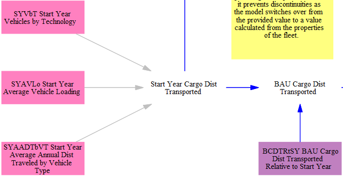
The EPS begins by determining the demand for transportation services, which is measured in units of cargo-distance, separated by vehicle type. Start year transportation service demand in the BAU case is taken in as the product of several input data variables: start year vehicles by technology, average vehicle loading, and average annual distance traveled by vehicle type. This demand is then modified in successive years by the input data variable for 'BAU cargo distance transported relative to start year,' as shown in the following screenshot:
Cargo distance transported is then modified for macroeconomic feedbacks from the Input-Output Model (see the Macroeconomic Feedbacks page), as shown in the screenshot below. We choose to modify freight travel by the weighted average percent change in industry's indirect and induced contribution to Gross Domestic Product.

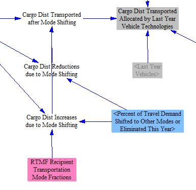
Next, we modify cargo distance transported by the Transportation Demand Management (TDM) policy lever, as shown in the screenshot below. TDM refers to a spectrum of different policies that generally attempt to reduce passenger usage of light-duty vehicles. These include improving public transit systems, zoning for higher density along transit corridors, zoning for mixed use neighborhoods and developments, building walking and biking paths, and congestion pricing and parking fees on light-duty vehicles. The effect is to decrease passenger usage of LDVs, aircraft, and motorbikes, while increasing passenger usage of HDVs (buses) and rail. The magnitudes of these effects are geography-specific and are customizable in the input data variable RTMF Recipient Transportation Mode Fractions.
TDM can also be applied to freight transport, which represents mode shifting and logistics. It decreases the freight ton-miles transported by HDVs (trucks) through better freight logistics and/or increases the freight ton-miles transported by rail.
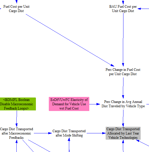
We also calculate how policy-driven changes in the cost of transportation services affects demand for those services by adjusting for the percent change in fuel cost per unit cargo distance. We determine the percent change in fuel costs by calculating the fuel cost per unit cargo distance in both the policy and the BAU scenarios.
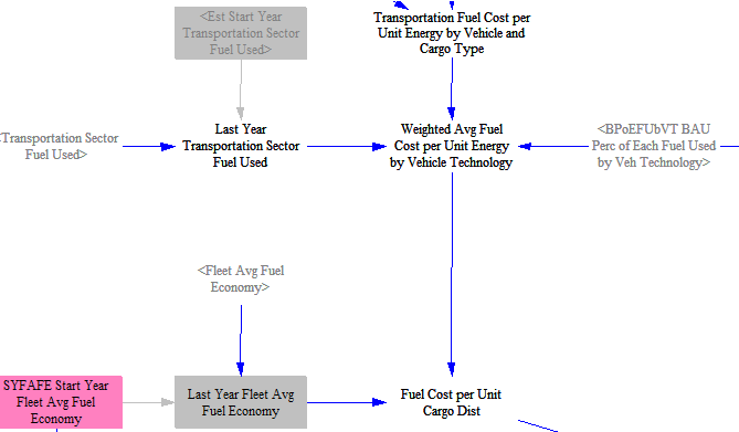
The model structure for the fuel cost per unit cargo distance in the policy scenario is shown in the screenshot below. The calculation for the BAU scenario mirrows this same structure, but using BAU versions of each variable. In both sets of calculations, we institute a one-year time delay to avoid circularity. For this reason, we need to read in input data for fuel economy of each vehicle type and technology in the start year (defined as one year before the first simulated year in the model). We then combine last year's transportation sector fuel used with the cost of transportation fuels used by each technology to determine a weighted average fuel cost per unit energy by vehicle technology. We then divide that quantity by the fleet average fuel economy of each vehicle type and technology to determine the fuel cost per unit cargo distance.
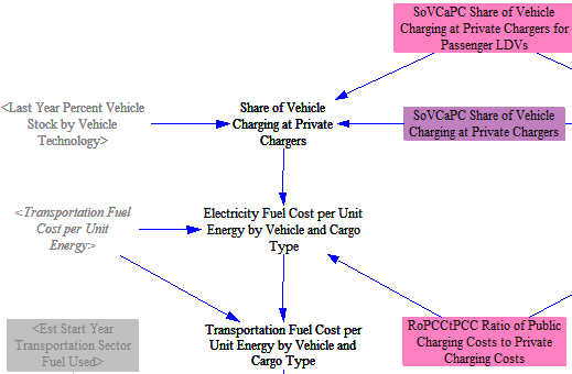
For non-electricity transportation fuels, the fuel cost per unit energy is the same regardless of which type of vehicle uses it. Electricity is a special case: the price an EV owner effectively pays per unit of energy depends on whether they charge at a private (home or depot) charger or at a public charger, and public charging is generally more expensive per unit energy than private charging. The model therefore tracks an electricity fuel cost per unit energy by vehicle and cargo type, blending the underlying electricity price with a public-versus-private charging mix and a 'Ratio of Public Charging Costs to Private Charging Costs' input. The private-charging share is set to one for vehicle types with dedicated depot charging (transit buses, freight rail, etc.); for passenger LDVs it is determined endogenously from a lookup against the BEV share of the existing passenger LDV fleet (sourced from a study of home charging access in the United States), so that as more EV households charge at home or in apartment garages the effective electricity price drifts toward the lower private rate.
We compare this figure with its corresponding BAU variable to determine the percentage change in fuel cost per unit cargo-distance that is attributable to the policies. Thus, policies that increase fuel cost will tend to make transporting cargo-distance more expensive, and policies that improve fuel economy will tend to make it less expensive. Literature on fuel economy improvements often discusses a "rebound effect," referring to the tendency to increase driving in response to the fuel savings that come from increased fuel efficiency. However, if increased fuel price is a driver of the increase in fuel economy, the "rebound" could be positive or negative, depending on whether the increased cost outweighs the increased efficiency, or vice versa. The 'Elasticity of Demand for Vehicle Use wrt Fuel Cost' is multiplied by the percentage change in fuel cost per unit cargo-distance to determine whether usage is increased or decreased, and by how much, for each vehicle type. We apply these changes to the the cargo distance after TDM effects to find the cargo distance transported in the policy case:
The final cargo distance adjustment in the model structure is to account for the 'Exogenous GDP Adjustment,' which is no longer used in the U.S. model. This feature can be used to adjust energy and service demand for the COVID-19 induced recession or other economic shocks that are not reflected in collected input data. Because the U.S. EPS input data already reflects COVID-19, we no longer rely on this feature. However, it is still in use in certain international EPS models.

Calculating New Cargo Distance Transported
Next, we must determine the share of the cargo distance transported that is attributable to new vehicles, meaning those purchased in the current model year. (This includes vehicles purchased to replace older vehicles as well as vehicles purchased that do not replace older vehicles and thus increase the total fleet size.) The cargo distance attributable to new vehicles sold in each year is seldom available as input data, and even in the cases where it is available, it does not always align precisely with the input data used to convert cargo distance to vehicles (average distance traveled and average passenger or freight loading). Accordingly, we use an input variable to assign a specific share of cargo distance each year to new vehicles. This value can be obtained roughly through input data sources or assumptions, but it needs to be calibrated, to prevent misalignment with other input data variables (as noted above) that can cause improper model behavior. Calibration typically shifts the shares only very slightly and is well within the error bounds of numerous underlying input data variables, and it likely improves model accuracy. For this variable, calibration is done by preventing sudden discontinuities in the numbers of retiring vehicles (of all technologies) at the model years that correspond to vehicle lifetimes:

Calculating New Vehicle Fuel Economy
Fuel Price Effects
The fuel economy of new (that is, newly sold) vehicles is modified based on four factors: fuel price, the R&D policy, the LDVs feebate policy, and the fuel economy standards policy. The following screenshot shows the calculation of the percentage change in fuel economy due to policy-driven changes in fuel prices:
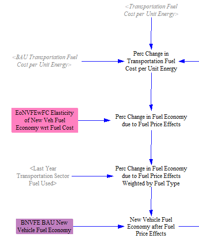
The cost of transportation fuels per unit energy is calculated on the Fuels page and referenced here. On the Fuels page, policies such as the carbon tax and fuel taxes can cause the fuel costs in the policy case to be higher than in the BAU case. On the "Transportation - BAU" sheet, we perform a similar calculation to obtain a corresponding BAU value. This allows us to compare the two values, obtaining a percentage change in fuel cost per unit energy due to our policy package. This change is combined with an elasticity of new vehicle fuel economy with respect to fuel cost, which reflects the behavior of both manufacturers (who may choose to make more efficient vehicles in response to fuel price increases) and the behavior of consumers (who will select more efficient vehicles from the available options offered by manufacturers at a given time).
Vehicle fuel economies are differentiated by vehicle type and vehicle technology, but not by the fuel used in a given vehicle type/technology combination. Accordingly, we obtain percent changes in fuel economy for each vehicle type/technology combination by weighting by fuel types used in each of these vehicles.
We then multiply these percent changes by the BAU new vehicle fuel economy (which is derived from input data).
Feebate
The feebate policy, which only applies to LDVs, has a specific effect on new LDV fuel economy based on the results of a study. We multiply the user's selected feebate setting by the effect of a feebate observed in that study to obtain the percent change in fuel economy due to the feebate, then apply that percent change to the new vehicle fuel economy:

Fuel Economy Standards
The improvement caused by the fuel economy standards policy is implemented directly as a percentage improvement to fuel economy (relative to BAU fuel economy in that year) for vehicles, with users able to differentiate by cargo mode and vehicle type. A further input data variable controls which vehicle technologies are subject to the standard. By default, this input data variable is set to apply fuel economy standards to only gasoline, diesel, and LPG onroad vehicles and diesel offroad vehicles in the U.S. The EPS does not currently allow users to select an emissions standard that would then be endogenously met through a combination of fuel economy improvements in internal combustion vehicles as well as an increase in the number of zero-emission vehicles sold. However, the separate Zero-Emission Vehicle Sales Standard policy (covered later in this documentation), or other policies that increase the penetration of zero-emission vehicles such as incentives can be applied in tandem with fuel economy improvements.

R&D
All R&D policies are defined as being additional to any R&D required to comply with other policies, such as tighter fuel economy standards. The user explicitly defines a desired improvement in fuel economy for new vehicles of each technology when setting the R&D lever.

Calculating NPV of Lifetime Vehicle Cost
In order to decide which vehicle technologies will be selected by purchasers to fill the need for new cargo-distance from a given vehicle type in the current year, the model needs to know the price of each vehicle technology as seen by purchasers. There are three components to this price: the upfront cost of the vehicle; the discounted lifetime cost of operating, maintaining, and -- for passenger-LDV battery electric vehicles (BEVs) -- installing home charging equipment for the vehicle; and a set of shadow costs applied to electric passenger light-duty vehicles to represent perceived non-monetary barriers (range anxiety, charging-station availability, and broader consumer preference factors). This section of the model calculates these costs and combines them into a single NPV of Lifetime Vehicle Cost, which is then converted to a per-mile cost for use in the vehicle choice function.
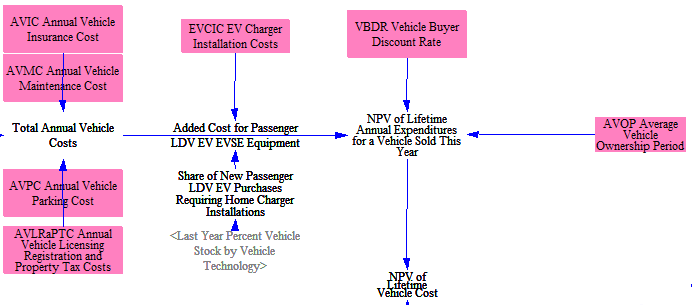
NPV of Lifetime Annual Expenditures
First, we take the average transportation fuel cost weighted by fuel type and multiply it by the technology-specific new vehicle fuel economy values we calculated earlier, giving us the fuel cost per unit cargo distance transported by each vehicle type and technology. As noted in the cargo-distance discussion above, electricity prices in this calculation are also differentiated by vehicle and cargo type to reflect the public/private charging mix.

Next, we convert this to fuel cost per unit vehicle-distance (for example, vehicle miles traveled instead of passenger miles traveled) using the average loading level of each vehicle type. We then multiply this by the average distance traveled by each vehicle type in a year to estimate the annual fuel expenditures to be expected for this newly sold vehicle in each year over the lifetime of the vehicle. (This is based on current model year fuel prices, not projections of future fuel prices. So in model year 2030, the fuel prices will be based on 2030 values, not on a series of values beginning in 2030 and ending in the last year of the vehicle's lifetime. This better reflects the decision-making process of purchasers with limited information about future prices.)

We then add in annual expected vehicle maintenance, insurance, parking, and licensing, registration, and property tax costs. Vehicle maintenance costs are differentiated by vehicle type and technology (as the cost to maintain an electric vs. a gasoline car, for example, can vary significantly), and other costs are differentiated by vehicle type only. These values are all read in as input data.
For passenger light-duty BEVs, we also add a one-time charging-equipment installation cost. Most EV buyers who do not already have a Level 2 home charger purchase and install one. The model multiplies a per-installation cost by the share of new passenger LDV EV purchases requiring an installation. That share is set to one minus the BEV share of the existing passenger LDV fleet, on the assumption that BEV buyers in households that already include a BEV typically already have a working home charger. The resulting installation cost adds to the NPV of Lifetime Annual Expenditures only for passenger LDV BEVs and is zero for all other vehicle/cargo/technology combinations.
Finally, we convert this stream of expected fuel and other expenditures over the vehicle's lifetime into a net present value (NPV) value, using an average vehicle ownership period and a discount rate adopted by vehicle buyers. We use an ownership period rather than vehicle lifetime as some vehicle types, for example freight trucks, are typically retained by the original buyer for a period much shorter than the vehicle's lifetime. A high discount rate is generally appropriate here, as vehicle buyers tend to undervalue future fuel savings (or costs) in their calculus of what vehicle to buy today. This is one of three factors that contributes to the NPV of Lifetime Vehicle Cost:
New Vehicle Price
The model adds these annual costs to the upfront price of the new vehicle. Prices for most vehicle technologies in future years are taken in as input data. For battery-equipped vehicles, we separately calculate the cost of the battery using endogenous learning curves -- their cost declines are linked to their cumulative deployment. An average battery pack price (in $/kWh) in the model start year is read from input data, and the price falls endogenously as calculated on the Endogenous Learning page. The starting price is treated as a passenger-LDV battery pack price; for other vehicle types and cargo modes, the model applies a 'Battery Pack Price Multiplier' (sourced from NREL's Annual Technology Baseline) to scale the price for freight LDVs, HDVs, and nonroad vehicles.
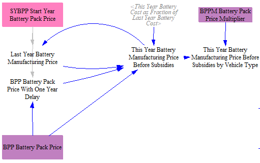
Subsequently, the model takes into account any subsidies for vehicle batteries. This section of code is built to reflect assumptions about the 45X advanced manufacturing tax credits from the U.S. Inflation Reduction Act. These credits offer a $45/kWh credit to producers for domestically produced batteries. The credit can be passed through to consumers in the form of lower upfront vehicle prices. However, we assume only a share is actually passed through. The model structure therefore has multipliers on the subsidy value for both the fraction of vehicle batteries produced domestically and the fraction of subsidy passed through to customers. This structure can be adapted to reflect battery manufacturing subsidies with their own requirements in other regions.
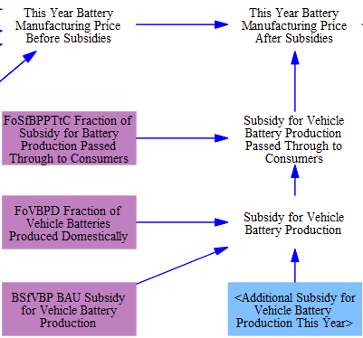
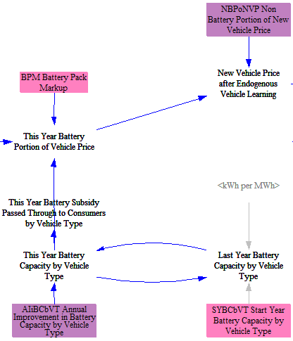
Next, the post-subsidy battery manufacturing price is converted to a retail-price-equivalent (RPE) basis by multiplying by a 'Battery Pack Markup' factor. This markup follows NREL ATB methodology, applying a retail price equivalent factor of 1.5 for light-duty vehicles and 1.2 for medium- and heavy-duty vehicles to estimate retail prices from manufacturing costs.
Lastly, the marked-up battery cost is converted from $/kWh to $/vehicle by multiplying by the battery capacity of each vehicle type, then added to the non-battery portion of new vehicle price. (reminder: for non-battery-equipped vehicles, this input variable is the full cost of the vehicle)
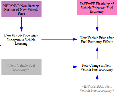
All vehicle prices are then modified based on differences in new vehicle fuel economy in the policy case relative to the BAU case and an elasticity of vehicle price with respect to fuel economy, to account for the increase in price due to more efficient car components. This is calculated separately for each vehicle type and technology, so we are comparing (for example) more vs. less efficient battery electric LDVs, not comparing battery electric and gasoline LDVs.
Next, we adjust the price of each vehicle technology for policy case R&D, if the model user has set one of these R&D levers to a non-zero value. After that, we account for the effect of the carbon tax on the cost of the vehicle itself (due to the embedded carbon in the vehicle- that is, the carbon that was emitted due to its construction).

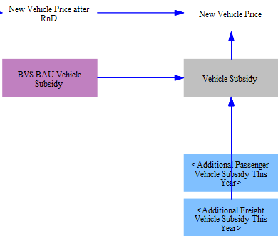
Finally, we adjust the vehicle price based on BAU subsidies and any additional subsidies that may have been specified by the user for this model run.
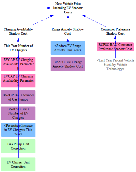
Shadow Costs for Electric Passenger LDVs
The third component of the NPV of Lifetime Vehicle Cost is a set of shadow costs applied only to electric passenger light-duty vehicles. These shadow costs are added to the calculated new vehicle price for the calculations determining which vehicles are purchased by consumers, but are not included in the actual costs tracked in the model's cash flow calculations. They are meant to represent perceived non-monetary barriers to EV adoption in consumer purchasing decisions. The model represents three such barriers as separate, additive shadow costs:
- Range anxiety shadow cost. Reflects buyers' concern about the distance an EV can travel between charges. Sourced from a Department of Energy study. A policy lever ('Reduce EV Range Anxiety') allows users to scale this shadow cost down.
- Charging availability shadow cost. Reflects the relative scarcity of EV chargers compared to gas stations. Calculated as a logarithmic function of the ratio of the projected number of EV chargers to the number of gas pumps; falls toward zero as charger deployment approaches parity with gas pump deployment. Affected by the EV Charger Deployment policy lever.
- Consumer preference shadow cost. Reflects broader non-monetary preference factors beyond range and charger availability — for example, perceptions of unfamiliar technology and concerns about resale value. Calibrated against historical light-duty vehicle sales data (see Forsythe et al., PNAS 2023 and the U.S. Energy Information Administration Annual Energy Outlook). The shadow cost decays as the BEV share of the existing passenger LDV fleet grows: it is multiplied by
1 − BEV share of last year's passenger LDV fleet, on the assumption that as more BEVs reach the road, the perception barriers represented by this shadow cost diminish.
The three shadow costs are summed with the new vehicle price and the NPV of Lifetime Annual Expenditures (the latter already including the EVSE installation cost described above) to produce the NPV of Lifetime Vehicle Cost variable:
New Vehicle Cost per Mile
The vehicle choice function described in the next section compares technologies in cost-per-mile units rather than in total NPV terms, so that vehicles with different annual usage patterns and different ownership periods can be compared on a like-for-like basis. We compute the New Vehicle Cost per Mile by dividing the NPV of Lifetime Vehicle Cost by the product of the average annual distance traveled, vehicle loading, and ownership period for each vehicle type, cargo type, and technology. This per-mile metric is used internally by the vehicle choice function; it is not exposed in cash flow tracking or in outputs outside the transportation sector.
Calculating Number of New Vehicles
Now that we know the New Vehicle Cost per Mile for each vehicle technology, we have the information we need to determine both the number of new vehicles and what technologies will be selected.
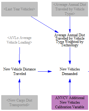
We begin by converting new cargo-distance transported to new vehicles demanded, using vehicle loading and annual average distance traveled by vehicle type (which were both used earlier to find annual fuel use per vehicle).
In some regions, changing economics and political factors cause the resulting historical-year sales to drift from observed values. We therefore include an optional, additive calibration adjustment, the 'Additional New Vehicles Calibration Variable,' to the new vehicles demanded by vehicle and cargo type. By construction, the calibration values across the historical time series sum to zero for each vehicle/cargo combination, so the adjustment shifts sales between years rather than changing the cumulative number of vehicles introduced.
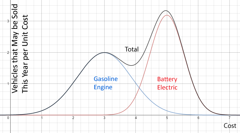
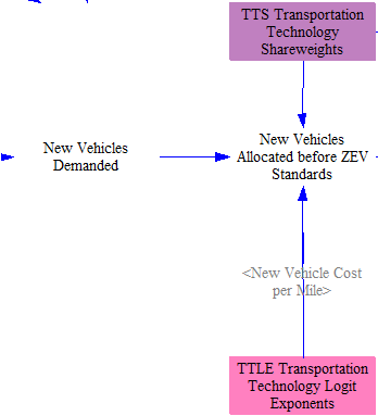
To determine what technologies of vehicle purchasers will buy (e.g. how many of the new passenger LDVs will be battery electric, how many will use a gasoline engine, etc.), we must allocate the demand by technology. We therefore need to implement a vehicle choice function, which we want to base on cost. However, we don't want to simply allocate all new vehicle demand to the cheapest option. While we track average vehicle costs in the model, in reality each vehicle technology spans a range of costs. The image below represents a simplified example of prices for gasoline engine and battery electric vehicles, where each technology has its own normal distribution with an unique midpoint on the cost axis (X-axis). The Y-axis is the quantity of vehicles of a given technology that can be sold in this year at a given cost. The volume inside these curves corresponds to a quantity of vehicles sold: cost (X) multiplied by quantity per unit cost (Y). We know the total amount of vehicles we need to sell, which is the volume under a portion of the black “Total” curve. Accordingly, demand is satisfied from left to right on the cost axis, filling in the volume under each individual vehicle technology's bell curve, until a total amount of volume has been filled in equal to the quantity of new vehicles needed this year. If this point is reached anywhere between the “3” and “6” numbers on the cost axis in the example diagram above, then a non-trivial number of gasoline engine vehicles and a non-trivial number of battery electric vehicles will be sold, and neither gasoline engine vehicles nor battery electric vehicles will be sold at the maximum possible rate this year.
We take a similar approach in the EPS by implementing what is known as a logit choice function. Its cost input is the New Vehicle Cost per Mile derived in the previous section. The function's behavior is controlled by two components. The first is a logit exponent, which determines purchasers' sensitivity to cost. The second is the technology shareweights, which can be calibrated based on historical sales. These shareweights capture non-cost factors such as consumer preferences, barriers to market entry, etc. The exponent and shareweight selections will determine the shapes and distributions of the curves for each vehicle technology. The following screenshot shows how this structure is implemented in the EPS:
After the cost-based vehicle allocation, we check to see if the share of zero-emission vehicles (ZEVs) meets the minimum required ZEV sales percentage in each subregion, which can be modified by two policy levers. Up to 60 subregions can be defined; in the U.S. model there are 51 regions, representing the states and the District of Columbia. The first lever allows the user to define non-BAU ZEV sales requirements for each subregion -- in the U.S. representing changes to the Advanced Clean Cars and Trucks rules of California and follower states. The second policy lever allows the user to define alternative, region-wide minimum sales shares -- in the U.S. this would represent changes to the Environmental Protection Agency's tailpipe standards for new vehicles.
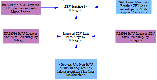
The vehicle technologies that qualify as ZEVs are determined through input data, and are set to EVs, plug-in hybrids, and hydrogen vehicles in the U.S. model. Users can also choose to change which vehicles qualify for the standard as part of a policy package with the Use Non BAU ZEV Qualifying Vehicles policy lever.

Before applying the standard, we calculate how many vehicles are sold in each subregion, then determine the share of vehicles that contribute to meeting the standard in each subregion based on user selected settings for which vehicles qualify. If the ZEV standard is met naturally, we keep the pre-ZEV standard allocation. Otherwise, we scale up ZEVs sales such that the standard is hit and scale down non-ZEV sales so as to avoid changing the total number of vehicles sold. This gives us the number of new vehicles by subregion.
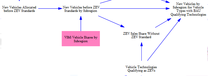
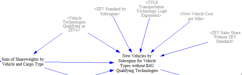
For some vehicle types -- typically off-road vehicles like ships and planes -- there are no ZEV-qualifying vehicles sold in the BAU scenario. As a result, the above approach does not work; we cannot scale up zero ZEV sales to meet a minimum sales share. For these vehicle types, we assume equivalent shareweights for all ZEV-qualifying technologies, allowing each technology (battery electric, hydrogen-fueled, etc.) to vye competitively for a share of the required sales. Each technology's New Vehicle Cost per Mile thus determines which technology will be sold to meet a minimum sales requirement.
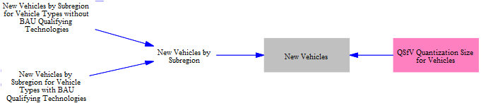
Finally, the number of vehicles of all types sold in each subregion are summed, applying a minimum quantization to account for rounding errors.
Tracking the Vehicle Fleet
Now that we know the numbers, types, and technologies of new vehicles sold this year, we are able to update the composition of the vehicle fleet (the total set of vehicles in the modeled region). The following screenshot shows the relevant structure:
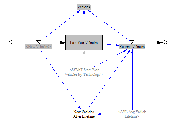
The composition of the vehicle fleet changes gradually over time, as more and more vehicles of various types and technologies are integrated into the fleet. Therefore, we use a level variable (one whose value is remembered from timestep to timestep and is affected by inflows and outflows) to track these vehicles. When vehicles retire (as their lifetimes are reached), they must be removed from the cumulative total. Although we have data on the starting number of vehicles in the fleet, we do not have their preexisting age distribution. Therefore, we assume that until the lifetime of a vehicle type is reached, the retiring fraction of the vehicles that existed before the first modeled year is one over the vehicle lifetime. Once a full vehicle lifetime has elapsed, the retiring vehicles are simply the New Vehicles that we introduced earlier, delayed by a number of years equal to the vehicle lifetime. This assumes that a vehicle's efficiency does not change significantly over the expected lifetime of the vehicle. This is generally true for typical vehicle lifetimes- a vehicle kept far beyond its normal lifetime might experience more degradation, but such vehicles are uncommon and are counter-balanced by vehicles that are removed from service before their normal lifetimes are reached (due to accidents, etc.).
Vensim doesn't update level variables with the current year's inflows and outflows; the current year's flows affect the level variable in the next year. We want to adhere to the user-defined policy implementation schedule without introducing a one-year delay. (If the user wanted a one-year delay, he/she would have put it into the policy implementation schedule.) Accordingly, we manually add the current year's inflows and outflows to the cumulative total to obtain the variable “Vehicles,” representing all vehicles in the simulated model year. We do something similar with all other level variables in the EPS.
Tracking Fleet Average Fuel Economy
We track changes in fleet average fuel economy by calculating the percentage change in fuel economy due to new and retiring vehicles each year, as shown in the screenshot below:
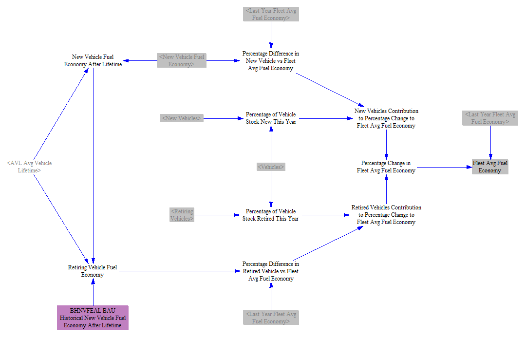
We first read in input data on historical new vehicle fuel economy (for example, if the average vehicle lifetime is 15 years, the fuel economy of a newly sold vehicle 15 years ago). After one vehicle lifetime, the retiring vehicle fuel economy is simply the new vehicle fuel economy delayed by one vehicle lifetime. We use this variable to find the retiring vehicle fuel economy and the percentage difference in this value vs. last year’s fleet average fuel economy. We similarly find the percentage difference in new vehicle economy. Because we know the number of retiring and newly sold vehicles this year, we can then calculate the contribution of each to the percentage change in fleet average fuel economy. Finally, we multiply this value by last year’s fleet average fuel economy to find the current year’s fleet average fuel economy.
Calculating Fuel Shifts Caused by the Low Carbon Fuel Standard (LCFS)
The next, large piece of the model calculates how the fuel used by each vehicle type and technology is affected by the low carbon fuel standard (LCFS), both a BAU LCFS (if any) and a policy case LCFS setting. There are multiple ways a LCFS policy could be defined, depending on how the policy is written. For purposes of the Energy Policy Simulator, it defines the percentage of energy used by vehicles that is free of carbon emissions (carbon-free energy, CFE), after an adjustment for the increased efficiency of electricity relative to fuels that are combusted. In the U.S. EPS, we follow the U.S. Environmental Protection Agency’s methodology and assign zero carbon emissions to biofuels, though users can edit this assumption through input data. Electricity has zero carbon emissions for purposes of the LCFS calculations (though the generation of electricity, which is handled in the Electricity Sector of the model, may result in carbon emissions there). Fuels are compared to the "reference fuel" for their vehicle type. For LDVs and motorbikes, the reference fuel is "petroleum gasoline," while for HDVs, it is "petroleum diesel." For example, if a particular biofuel gasoline has 50% of the carbon intensity of petroleum gasoline, then half of the energy in that fuel would be considered CFE and half would not.
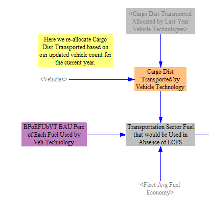
The first step is to determine the amount and types of fuel that would be used in the transportation sector in the absence of an LCFS policy. We take in the percentages of fuel used by different vehicle technologies, which is only relevant for certain technologies. Gasoline engine and diesel engine vehicles can burn either petroleum fuels or biofuels, while plug-in hybrids can consume electricity, a petroleum fuel, or a biofuel. Other vehicle technologies only consume a single fuel type. We multiply these percentages by the total cargo-distance transported by each vehicle type and technology, as well as by the fleet average fuel economy, to obtain total quantities of fuel.
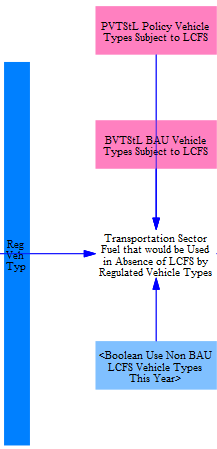
Next, we filter out vehicle types that are not regulated under the LCFS policy. This can be customized through an input data variable or adjusted in a policy scenario using the non-BAU LCFS vehicle types lever and input data. For the U.S., we filter out aircraft so that they neither are bound by nor contribute to satisfying the LCFS. For visual clarity, the model separates regions of the structure that are subject to filtering by vehicle type behind blue bars.
Next, we make an adjustment for the efficiency of electricity. Electricity is converted into the mechanical motion of a car much more efficiently than combustible fuels are converted into motion. If we don't account for this, the quantity of electricity used will be very small, making it hard to satisfy an LCFS requirement based on raw CFE. Therefore, we work in units of electricity that have been adjusted to have the same efficiency as the combustible reference fuels (gasoline or diesel). This allows us to calculate LCFS compliance more simply, and we undo the adjustment at the end of the calculations, so we ultimately demand the correct amount of electricity. For visual clarity, the model separates regions of the structure that are subject to the electricity efficiency adjustment behind orange bars.

Next, the model converts fuel types to CFE. Reference fuels (petroleum gasoline and petroleum diesel) have zero CFE. Every other fuel has an amount of CFE equal to its carbon intensity ratio (relative to its reference fuel) multiplied by the amount of that fuel being used. For visual clarity, the model separates regions of the structure that are working in CFE units behind green bars.
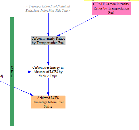
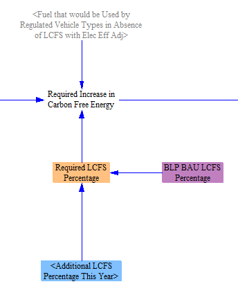
Next, we calculate the required increase in CFE by comparing the amount of CFE prior to application of the LCFS (as a fraction of the energy in fuel used by regulated vehicle types after electricity adjustment) with the required LCFS percentage. The required percentage is the sum of any BAU LCFS percentage and any user-specified policy case LCFS percentage.
Next, we need to determine the quantity by which CFE may be increased from shifting to each eligible fuel for each vehicle type and vehicle technology. To do this, we begin by taking in (as input data) the maximum percentage of each fuel that is usable by each vehicle technology. The model provides this input as separate BAU and non-BAU CSV files for every supported vehicle/cargo/technology combination. A policy lever ('Use Non BAU Max Fuel Consumption by Veh Type') allows users to apply the non-BAU set of maximums in policy scenarios, which is useful when modeling regulatory or market changes that expand the share of biofuels, hydrogen, or electricity that a given vehicle technology can accept. We convert this to percentage points of fuel increase relative to the BAU percentages, then we apply the same three filters or conversions applied to the fuel that would have been used in the absence of an LCFS. That is, we filter out non-regulated vehicle types, adjust for electricity efficiency, and convert to CFE. We then use this quantity to divide, proportionally, the required increase in CFE by vehicle type and by fuel. (We make a small adjustment to correct for the fact that plug-in hybrids could shift their petroleum fuel consumption to either electricity or biofuels, to avoid exceeding the total quantity of energy that may be shifted.)
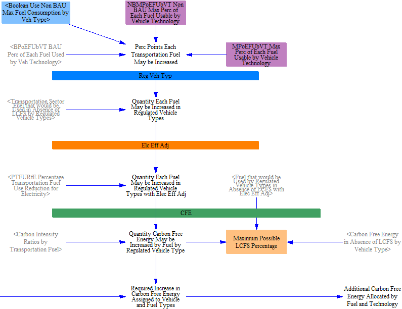
We then assign the CFE increases to vehicle technologies, which can be done explicitly based on the known fuel and vehicle types.

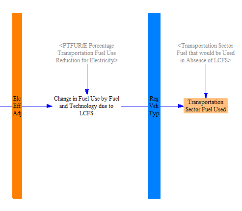
Finally, we sequentially reverse the three filters/adjustments undertaken earlier that allowed us to work in terms of the necessary quantities. First, we convert back from CFE to energy, and we apply negative shifts to the reference fuels equal in magnitude to the positive shifts in the low-carbon fuels, to preserve the same quantity of energy use (keeping in mind that the electricity efficiency adjustment is still in effect, artificially making its efficiency equal to that of the other energy sources, so we can shift between them accurately).

Next, we undo the electricity efficiency adjustment. This reduces the quantity of electricity used back to its true value (after the LCFS effects). Finally, we add in the fuels assigned to the non-regulated vehicle types (aircraft in the U.S. model), which are part of the total fuel used in the transportation sector but were exempted from the entire LCFS calculation process. This results in the final value of total fuel used.
Note that while the methodology to calculate the effects of the LCFS policy accounts for electric vehicles’ contribution to meeting the standard, it does not endogenously deploy additional electric vehicles. Instead, it only shifts the fuel types used within existing vehicles.
Calculating Emissions and Electricity Use
We convert the fuel use of known fuel types into emissions, by applying Transportation Sector emissions intensities by fuel. We break this calculation into two parts to account for the fact that some of the twelve pollutants tracked in the model are separately regulated for vehicles. In the U.S., we consider all non-GHGs (VOCs, CO, NOX, PM10, PM25, SOX, BC, and OC) to be separately regulated, meaning changes in fuel economy do not necessarily lead to changes in the emissions of these pollutants per mile traveled. That is because vehicle manufacturers may design vehicles to meet fuel economy and conventional pollutant standards separately to narrowly comply with each standard. Users may apply the Conventional Pollutant Standard to address these separately regulated pollutants.
The emissions intensities for each pollutant are calculated on the Fuels sheet, which is covered on the Fuels page of the documentation. Emissions of separately regulated pollutants are calculated by multiplying the emissions intensities by the amount of fuel used, accounting for any changes in emissions intensities from the Conventional Pollutant Standard policy. Emissions of all other pollutants are calculated by multiplying the amount of fuel used, the emissions intensities, and the percent change in the fleet average fuel economy.
Transportation sector electricity use is broken out separately and converted to MWh (no efficiency adjustment is needed here, because we are already working in units of electricity- this is a strict unit conversion from BTU to MWh). This is summed with other sources of electricity demand to provide an input to the Electricity Sector.

LCFS Credit Estimates
Some jurisdictions, such as California, use the concept of an "LCFS credit" in their LCFS legislation. The EPS does not work in this type of unit directly, preferring instead to use CFE and decarbonization percentages, as these units are more fundamental and related to physical quantities than LCFS credits. However, to improve the utility of the model for regions that do use an LCFS credit methodology, this section performs calculations that estimate some costs related to LCFS credits.
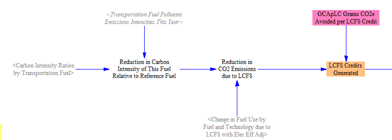
We first calculate the reduction in CO2 emissions due to the LCFS policy using the previously calculated change in fuel use due to the LCFS and difference in carbon intensities of each fuel type relative to the reference fuel. We then multiply this value by input data on the grams of CO2e avoided per each credit to find the total number of LCFS credits generated.
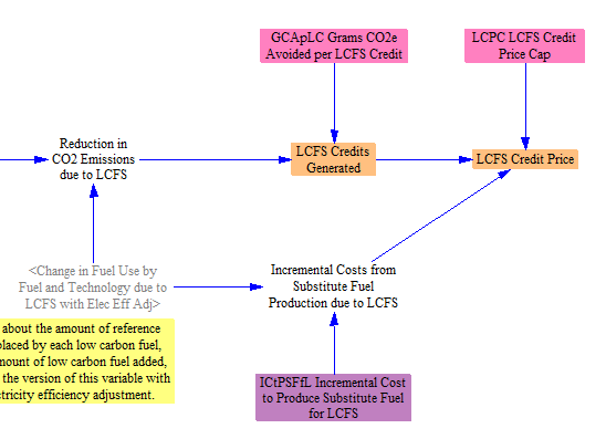
Finally, we find the resulting LCFS credit price. The price of an amount of low-carbon fuel needed to generate one LCFS credit buys two things: the credit itself, plus the fuel (to do useful work). The value of each low-carbon fuel is estimated via the value of the energy-equivalent amount of its corresponding reference fuel, as they can perform the same work. Accordingly, the LCFS credit value is based on the increment between the costs of the low-carbon fuel and the energy equivalent amount of its reference fuel. (Note that this involves a simplification, as the ease of using the underlying fuel in vehicles is not taken into account. For example, it is easier to use diesel than an energy equivalent amount of natural gas due to the fact that most existing HDVs are designed to use diesel.)
We take in input data on the incremental cost to produce a unit of fuel used to meet the LCFS (compared to the reference fuel). This is multiplied by the change in fuel use to find the incremental costs of fuel production. Finally, we calculate the LCFS credit price as the minimum of either a price cap (if one exists), or the incremental costs divided by the number of LCFS credits generated. (In practice, whether or not the cap is "reached" in each year would depend on whether or not there was potential in that year to obtain the required number of LCFS credits from the fuel types capable of generating these credits at a cost below the cap.)
This page was last updated in version 4.0.5.