Electricity Sector (cash flow)
The "Electricity Sector - Cash Flow" tracks changes in cash flows in the electricity sector, covering all aspects of the electricity supply system and industries it affects. This includes cash flows for spending on fuel, construction and retrofitting, subsidies, carbon transportation and storage, operations and maintenance, demand response, imports and exports, transmission and distribution capital and operating costs, and costs of various market mechanisms, such as the wholesale energy market or the capacity market. Changes in cash flows are used to estimate changes in revenues and expenditures across different industries as well as to compute changes in the costs of delivering electricity to consumers.
Cost Components
Generation Construction Costs
The following model structure calculates the changes in cost due to construction and retrofitting of electricity generating facilities:
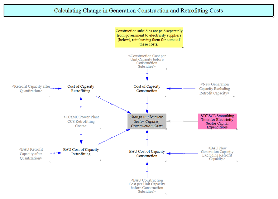
The construction cost per unit capacity before subsidies is the same for most technologies in the BAU and policy cases. However, certain plant types subject to endogenous learning (covered in the Endogenous Learning sheet) can have policy driven capital cost declines. Differences in spending on generation and retrofitting costs arise from different quantities and types of power plants being constructed in each scenario as well as the extent to which endogenous learning changes the unsubsidized capital costs.
The costs in each case are subtracted from each other, and an averaging function in Vensim (set to a 3-year averaging time) is used to even out unrealistic spikiness that comes from dramatically different amounts of capacity being built in adjacent years. Three years was chosen as a compromise between more averaging and avoiding the average in of too many "zero" values from beyond the model run period (a shorter timeframe) and is a fair approximation of the average time to build new power plants (though this varies widely across different power plant types).
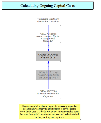
Ongoing Capital Costs
Existing power plants have ongoing capital costs beyond O&M costs. For example, nuclear plants need somewhat regular capital investment to maintain safety. We track ongoing capital costs for the existing fleet by multiplying the surviving capacity by a power plant type specific weighted average annual capital cost per unit capacity to find the change in ongoing capital costs. These ongoing capital costs are tracked separately from the vintage-based recovery of historical construction financing described above.
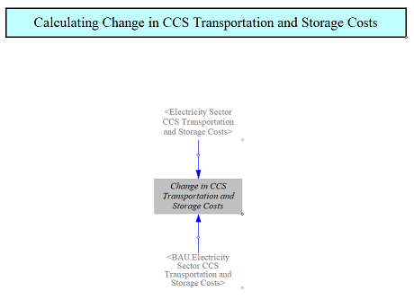
CCS Transportation and Storage Costs
We also track changes in the costs to transport and store CO2 that has been captured at plants equipped with CCS. Spending on CO2 transportation and storage costs is calculated on the CCS page and the electricity CCS portion of those costs in BAU and policy cases is compared to determine the change in costs.
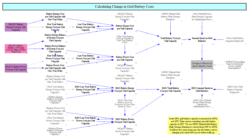
Spending on Batteries
The model determines the change in expenditures due to the construction of grid batteries and batteries at hybrid power plants. Batteries are one of the technologies for which the model endogenously calculates cost declines based on total global deployment. The cost declines are based on the number of doublings of battery capacity relative to the start year, as discussed in the Endogenous Learning code. Battery costs are broken into energy costs, power costs, and balance of system costs.
We find the difference in total new capacity of deployed battery storage in both the BAU and policy cases to determine the change in battery storage built this year. This is multiplied by the cost of batteries per unit capacity, which is calculated here based on the endogenous learning calculations. The structure is as follows:
Fuel Costs
The following model structure calculates the change in cost, fuel industry cash flow, and taxes paid due to spending on fuels:
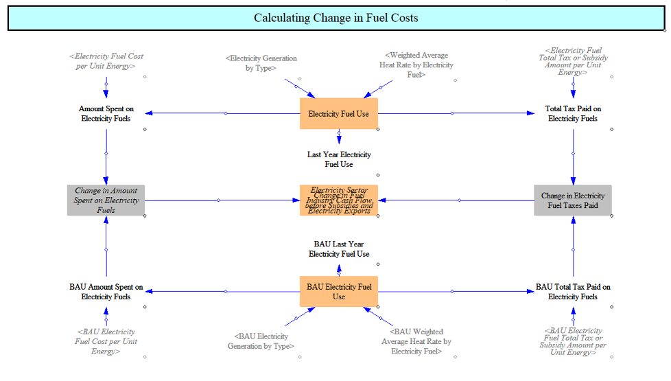
For each of the BAU and policy cases, we find the quantity of fuel consumed to supply electricity by multiplying the electricity generation (by power plant type) and the weighted average heat rate (efficiency) of power plants. Heat rates for CCS equipped plants reflect the lower efficiency of those plants.
We find the total amount of money spent on electricity fuels (including taxes) by multiplying the amount of fuel consumed by the fuel cost per unit energy. We find total taxes paid on fuels by multiplying the quantity of fuel consumed by the amount of fuel tax per unit energy. The difference in amount paid between the BAU and policy cases gives the change in amount spent on electricity fuels, which we use to track changes in cash flows to fuel suppliers. The difference in amounts of taxes paid gives the change in taxes, which will be assigned to government. Taking the difference in amount spent minus the difference in taxes paid yields the change in cash flow for the fuel industry (disaggregated by fuel, because we break down this industry into more meaningful industry categories on the Cross-Sector Totals sheet).
Generation O&M Costs
The model compares both fixed and variable O&M costs using the structure shown in the screenshot below:
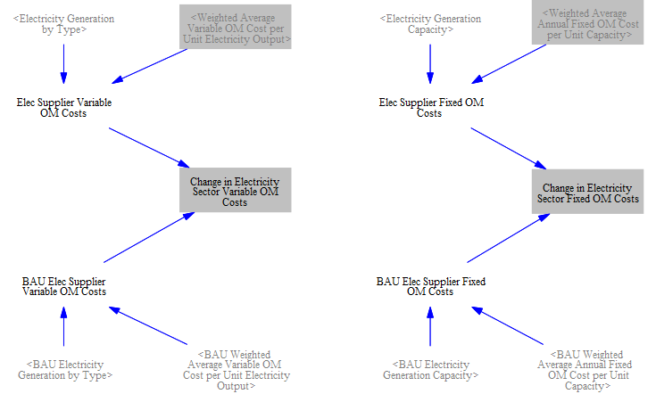
The differences in O&M costs derive from different amounts of capacity of each power plant type and different amounts of power generated by each power plant type in the BAU and policy scenarios. We take the quantities of capacity and generation straight from the "Electricity Sector - Main" and "Electricity Sector - BAU" pages. Taking the difference between the sums of the BAU and policy O&M costs yields the overall change in O&M costs due to the policy package.
Rebate for Sequestered CO2
In the event that there is a carbon price in BAU and/or the policy scenario, electricity suppliers receive a rebate, i.e. some positive cash flow, for sequestering CO2, as shown in the following structure:
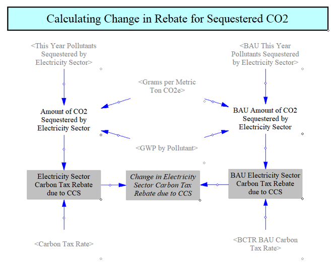
First, we convert the amount of CO2 sequestered from grams of pollutant to metric tons of CO2e. (Although "This Year Pollutants Sequestered by Electricity Sector" is subscripted by pollutant, only CO2 has a non-zero value for its amount of sequestration.) We multiply this by the carbon tax rate to determine the "rebate" received for sequestering the CO2. In reality, electricity suppliers are likely to have to pay carbon prices, so this "rebate" is merely a lowering of electricity suppliers' carbon pricing bills, rather than a net payment of money from government to electricity suppliers.
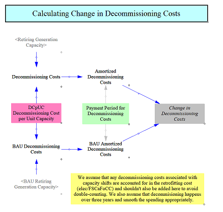
Decommissioning Costs
When power plants are retired, they have to be decommissioned. We track changes in spending on decommissioning costs. We compare the retiring capacity in the BAU and policy scenarios and multiply these by a power plant type specific decommissioning cost per unit capacity. We average these costs over a fixed set of years (3 years in the US EPS) assuming that decommissioning takes some amount of time to occur. We then compare these values for BAU and policy to get a total change in decommissioning costs.
Generation and Grid Battery Electricity Supply Subsidies
Qualifying power plants may also receive a subsidy per unit of electricity generation. We use Vensim's stock and flow structure to track the eligibility of new and retrofit capacity for generation subsidies over time. In the BAU, we assume subsidies are paid for ten years after the construction of each power plant. We then take the difference between the policy and BAU generation subsidies paid to feed into expenditure and revenue tracking.
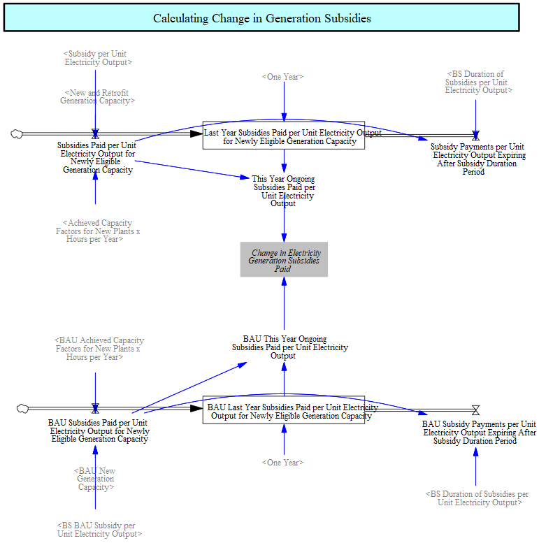
In addition to subsidies for new and retrofit capacity, users can apply a production subsidy to existing plants, specified per unit of output for each electricity source. This is combined with any business-as-usual existing-plant subsidy (after applying the Reduction in BAU Subsidies lever) to give a total subsidy per unit output for existing plants. The model converts this per-output value to a per-capacity basis using each source's prior-year capacity factor, and the result feeds the plant revenue used in the retirement and capacity-expansion calculations.
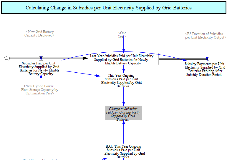
A similar structure is used to track subsidy payments for electricity supplied to the grid by batteries.
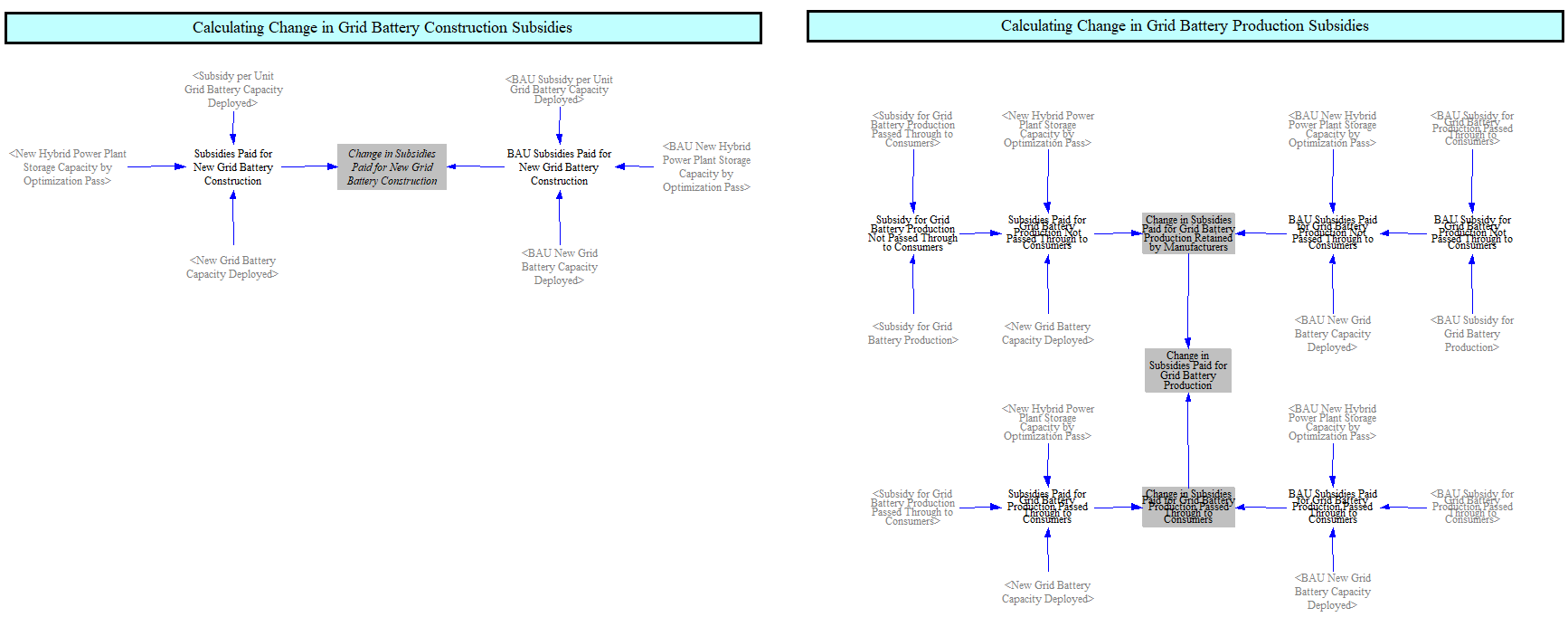
Other Grid Battery Subsidies
We also track two other categories of spending on grid battery subsidies: subsidies for production of grid batteries (paid to manufacturers), and subsidies per unit capacity installed (paid to electricity suppliers).
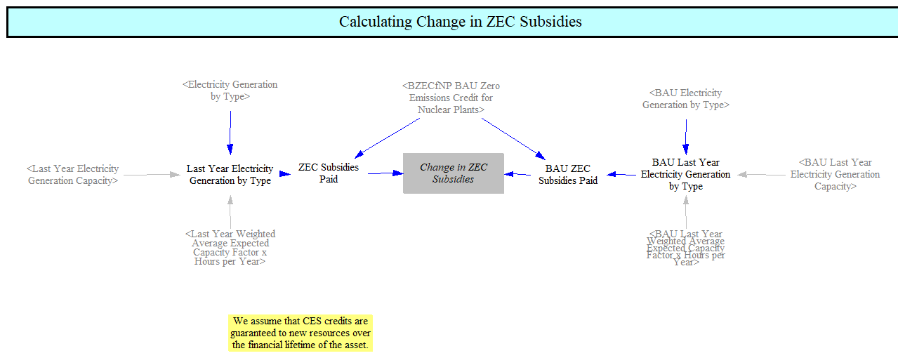
Zero Emission Credit Subsidies
Some regions, for example some US states, have additional subsidies for specific power plant types, such as nuclear power plants, often called Zero Emission Credits (ZECs). We calculate the change in these subsidy payments but comparing qualifying generation and subsidy amounts in BAU against the policy scenario calculations.
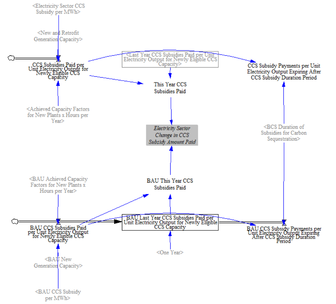
Construction and CCS Subsidy Payments
The following structure handles differences in construction subsidies for new and retrofit capacity caused by the policy package:
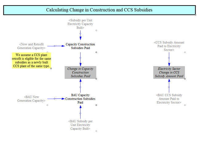
In the BAU case, capacity and CCS retrofit subsidies are applied based on BAU new and retrofit capacity. In the policy case these subsidies can be affected by multiple policies (which change the subsidy amounts) and the amount of capacity receiving incentives that is deployed. The change in capacity construction and CCS subsidies reflects differences in subsidy levels and new and retrofit capacity.
This section also calculates the change in CCS subsidy payments based on the amount of CCS-equipped new or retrofit capacity in each timestep and the subsidy duration.
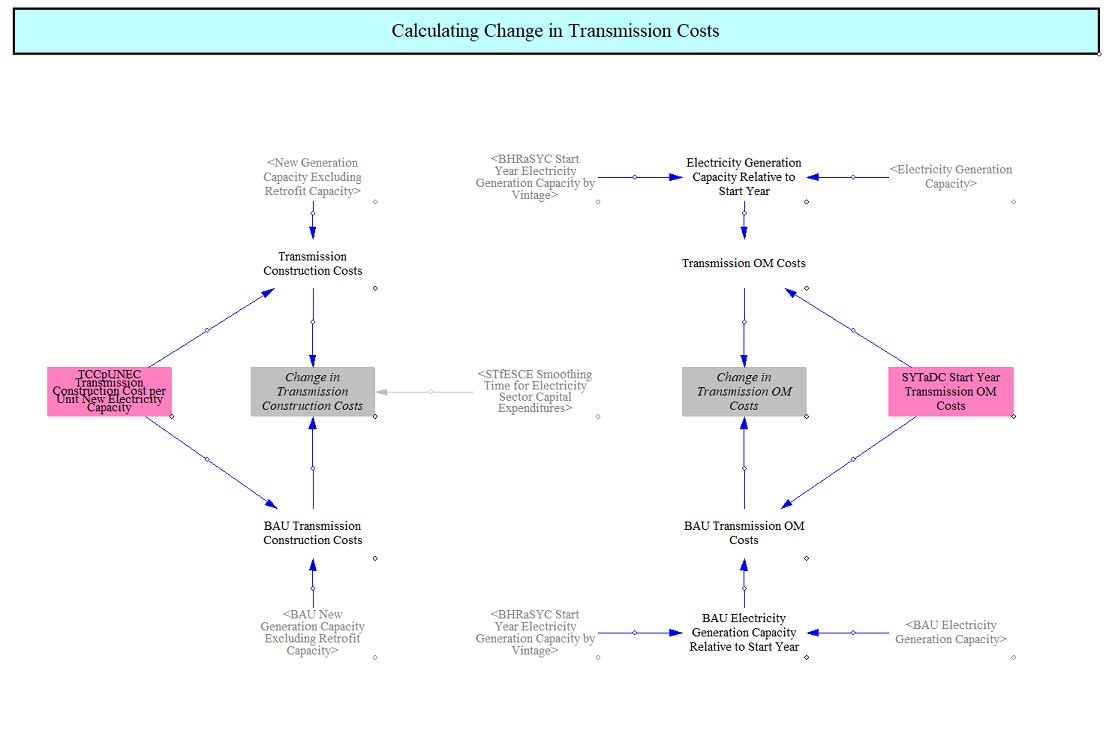
Transmission System Costs
Transmission deployment is endogenously estimated in the EPS and the model tracks changes in spending on transmission capital and transmission operating maintenance costs. Input data specifies the cost of new transmission construction per unit new capacity of various power plant types. This data is multiplied by the new construction of power plants to determine new spending on transmission capital. These values are averaged over several years, defined in input data, to reflect the time period over which it takes to physically construct transmission. Costs are compared between BAU and policy cases to determine the change in spending on transmission construction.
Transmission operating and maintenance costs are calculated based on the growth in total electricity generation capacity. Input data defines transmission O&M spending in the start year, and in subsequent years this spending increases based on the growth in electricity generation capacity.
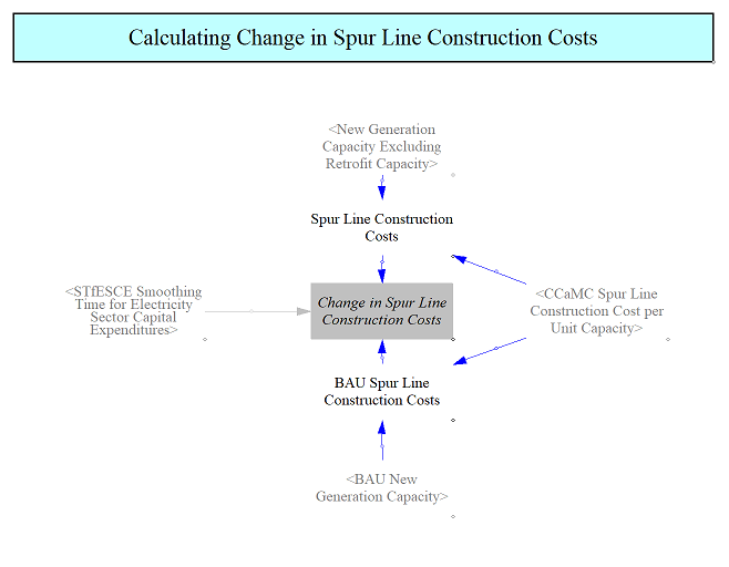
Spur Line Construction Costs
The EPS includes estimates of spur line costs, or the cost of running lines from a power plant to the bulk transmission system, in cash flow estimates. These costs are defined in input data and can vary by power plant type. Each power plant type can have an associated cost, in $/MW, that gets multiplied by new capacity to estimate the total spending on spur lines for each power plant type. These costs are averaged out over a set number of years, defined in input data, to avoid spikiness, and to reflect the fact that, like power plants, spur line construction often takes place over a duration exceeding a year.
Distribution System Costs
Distribution system investment is endogenously modeled as a function of peak electricity demand. Capital costs are estimated based on the increase in peak load multiplied by a cost per unit increase in peak load. Operations and maintenance costs are similarly estimated, using start year costs and growing or shrinking these in future years based on the change in peak load. Peak load is defined as total electricity demand after adjusting for onsite generation, which can often reduce peak load.

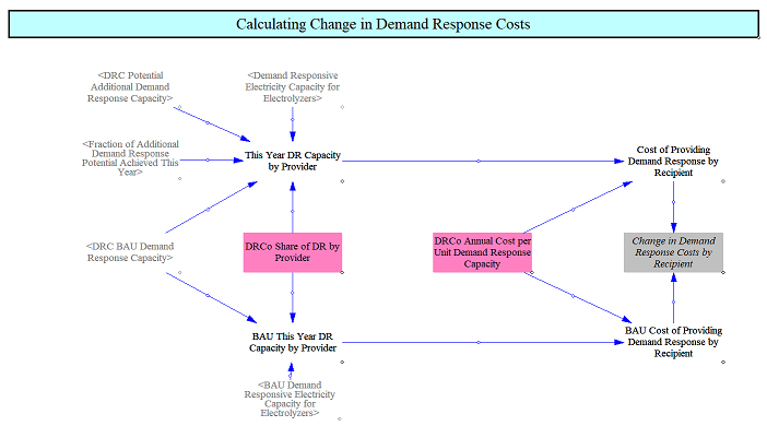
Demand Response Costs
The model tracks deployment of demand response capacity in the BAU and policy cases and tracks changes in spending on demand response across both scenarios. We sum the total demand response capacity across both scenarios, which is driven by input data and policy levers and allocate this across different providers, notably industries and consumers/labor, which reflect the building/facility types providing the DR for cash flow tracking purposes. We then multiply by this by a capacity cost per unit DR capacity to estimate the total spending on DR across BAU and policy scenarios and compare these values to find the change. DR is assumed not to have any operating costs but rather only have capital costs.
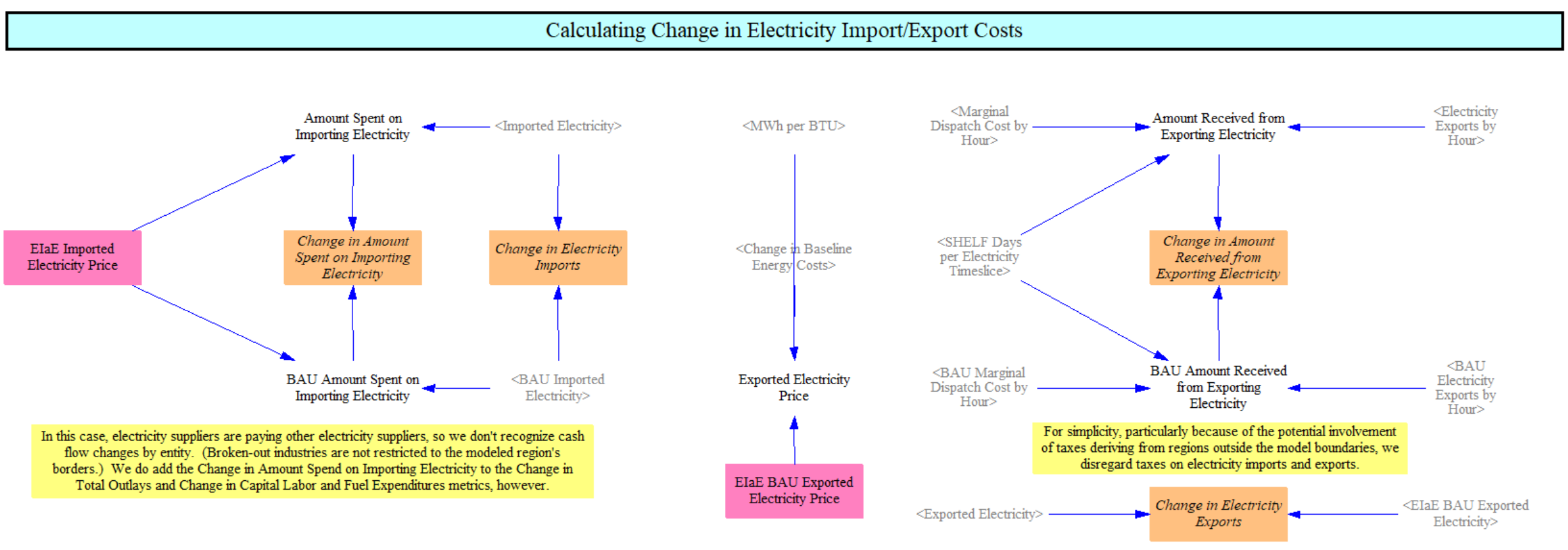
Electricity Import and Export Costs
The model also calculates the amount spent on buying electricity (from beyond the borders of the modeled region) and selling electricity to entities outside the borders of that region. For imports, we estimate the price of electricity as sold by entities beyond the model borders via input data specifying imported energy market prices.
We multiply the price of imported electricity by the amount imported in the BAU and Policy cases, then take the difference to find the change in amount spent on importing electricity.
For exports, we do something very similar, except that we adjust the exported electricity price by changes in the calculated electricity market prices in the model. This step is required because in BAU and policy scenarios where a lot of low marginal cost clean energy is deployed, the market price can drop significantly, and the export price should reflect changing market prices.
In the future, we hope to make imports and exports more dynamic and to calculate prices endogenously.
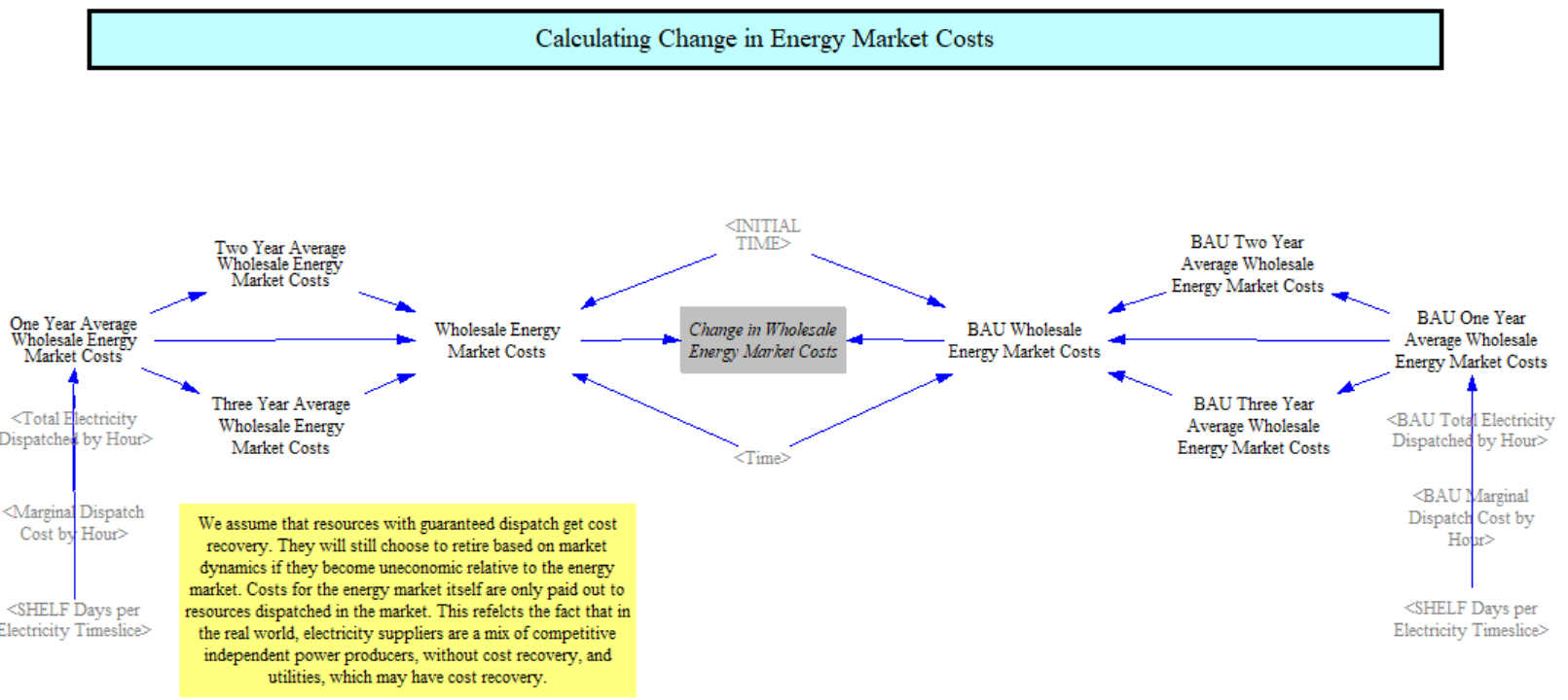
Energy Market Costs
Annual energy market costs are calculated in the EPS. These costs are calculated using the hourly marginal dispatch costs calculated on the Electricity Sector Main tab. They reflect the marginal hourly dispatch costs across the entire electricity system. Total costs are estimated by multiplying least cost dispatch and the market price in each hour, then summing over the year. Costs for resources dispatched under guaranteed dispatch, the portfolio-standard qualifying dispatch mechanism (covering both RPS- and CES-qualifying resources), and the zero or negative dispatch cost mechanism are not included here, because it is assumed these resources have fixed contracts and guaranteed cost recovery. For example, many clean energy projects have power purchase agreements (PPAs) in which a price per megawatthour is agreed upon, with excess revenue credit back to the developer and shortfalls in revenue being made up by the offtaker (the purchaser of the power).
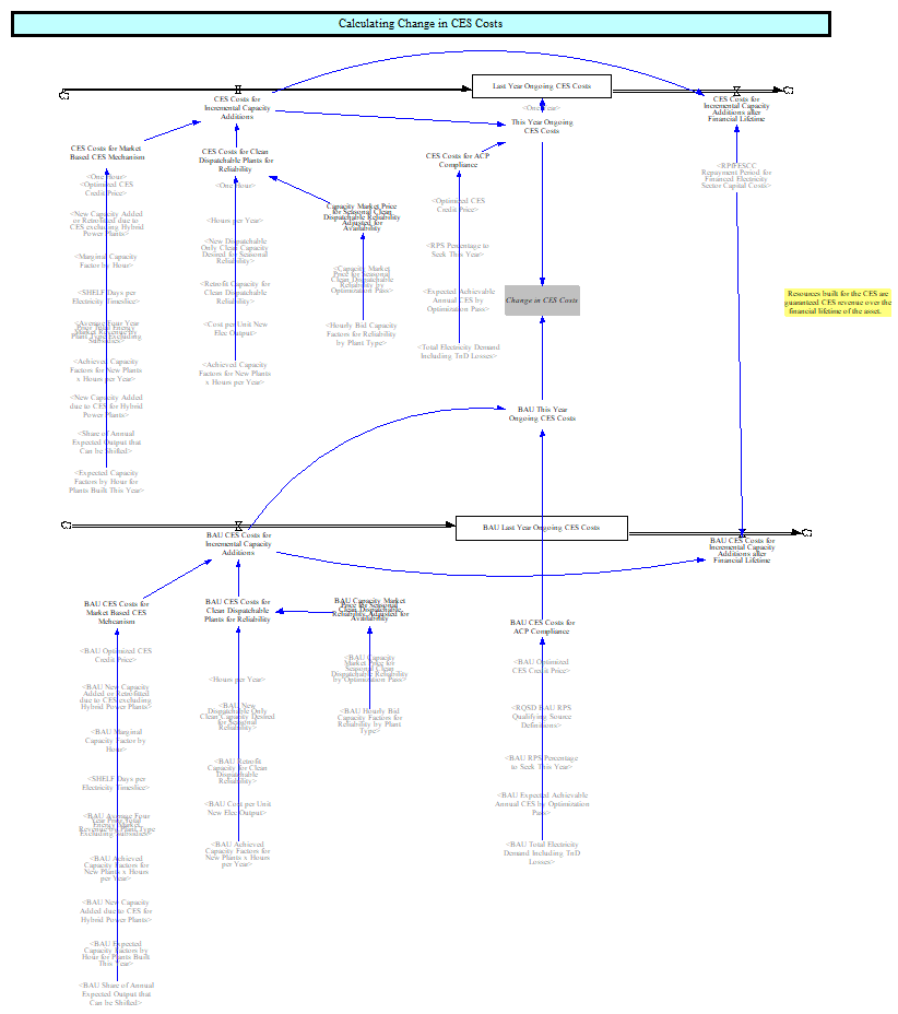
Clean Electricity Standard Costs
The EPS includes a unified portfolio-standard mechanism that can simultaneously enforce a Clean Energy Standard (CES) and a Renewable Portfolio Standard (RPS). This mechanism is discussed fully on the Electricity Sector Main page but reviewed here. Each portfolio standard computes its own credit price that drives sufficient incremental qualifying generation, and the cost calculations described below are performed separately for the RPS and CES paths and then aggregated. The total costs of the market-driven portfolio-standard component, which includes both credit costs and the required revenue for qualifying resources, are calculated in the "CES Costs for Market Based CES Mechanism" variable (despite its name, this variable covers both RPS and CES paths). Costs are estimated by multiplying the output of qualifying plants by the credit price and the market revenue that would have been received. We assume that in each year the qualifying resources enter into a contract for their electricity as the sum of the credit price and the anticipated market revenue, i.e., that the credit price is guaranteed to those resources over the financial lifetime of the asset. The portfolio-standard mechanism also includes hybrid resources. When energy market costs are calculated (discussed above) they do not include these resources to avoid double counting the revenue.
Additionally, as the CES approaches 100%, the EPS engages a mechanism to ensure sufficient clean firm/flexible capacity is available. The amount of capacity required and the threshold at which this requirement is triggered are determined by input data. As with the market based CES mechanism, it is assumed that these credits are made available at a fixed amount for the financial lifetime of the asset. These costs are estimated by first finding the market price and then multiplying it by the capacity deployed under this mechanism.
These costs are fed into a stock and flow structure to reflect their availability during the lifetime of the assets and track the total change in costs of a CES program over time. After the financial lifetime, the credits expire and the costs are reduced.
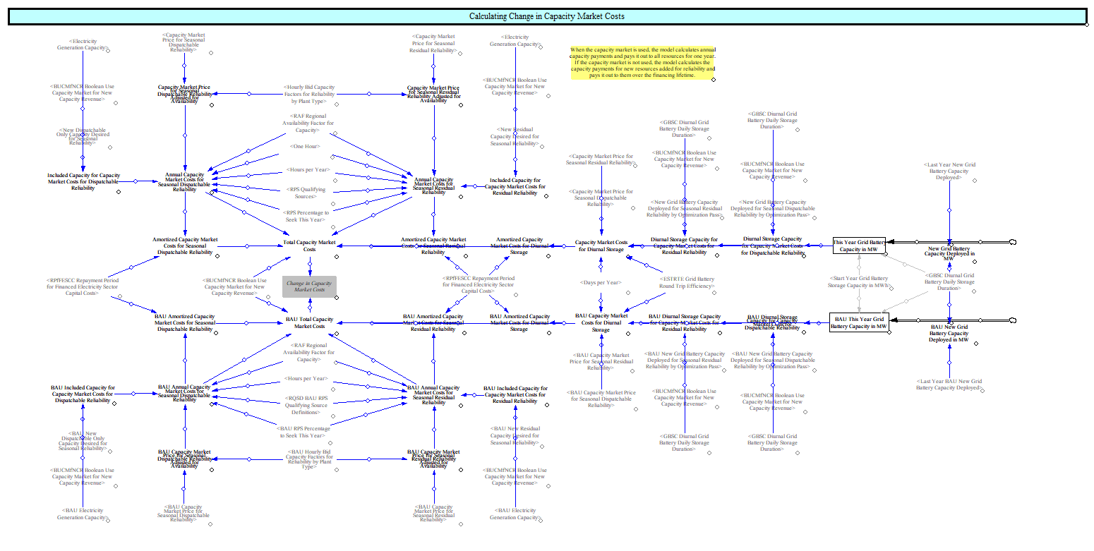
Capacity Market Costs
The EPS includes a capacity mechanism to ensure sufficient capacity is available for periods of peak demand and limited resource availability. As outlined on the Electricity Sector Main page, the model computes a capacity price during each of the two reliability passes (the clean-dispatchable-only pass and the all-resources pass), based on the single binding peak hour identified in that pass. Computed capacity payments are paid out to qualifying resources, adjusted for their availability during the binding hour of the mechanism. Capacity prices are recalculated every year and only paid out on a yearly basis. This approach is meant to approximate a market-based capacity construct.
A control lever setting allows the use of an alternative method. When this toggle is enabled, the capacity price is calculated similarly but only paid out to resources built in that year specifically for reliability purposes. The model assumes that the capacity payment is fixed annually for the financial lifetime of the asset being built. This approximates a different kind of market construct, such as a tolling agreement or the way in which a vertically integrated utility might contract for capacity over many years. This approach reduces the annual cost of the capacity mechanism but can lead to higher long-term costs, depending on the specifics of the capacity need in the model region.
Battery storage is integrated into the capacity mechanism and payments follow the same structure, depending on whether the control lever is enabled.
The structure below covers calculation of these costs for both approaches and for both traditional resources and battery storage resources, across both reliability passes.
When the RPS/CES policy lever is set to a value of 100%, non-qualifying resources lose their eligibility for the capacity market, and this section includes variables and code to ensure that dynamic is captured.
Allocating Changes in Expenditures and Revenue
Changes in Expenditures
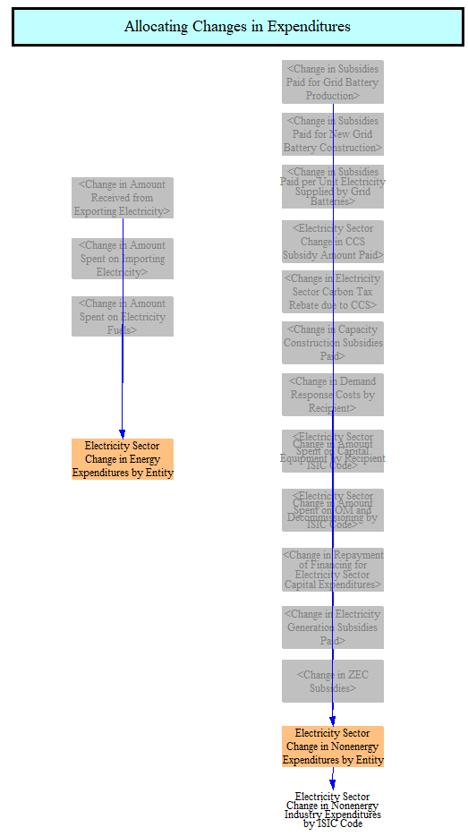
Now that we have calculated the changes in spending for the electricity sector, we need to assign those costs to the corresponding cash flow entities, as well as their corresponding ISIC codes (to be used in the Input-Output Model).
First, we allocate changes in energy expenditures. We track net changes in expenditures for foreign entities importing and exporting electricity. We estimate the net change in spending on electricity fuels and imports and assign this to the electricity suppliers cash flow entity.
Next, we allocate change in nonenergy spending by entity and ISIC code. For cash flow entities, all costs are allocated either to government, electricity suppliers, or nonenergy industries. Government costs include all subsidies and tax rebates. Nonenergy industry costs include all of the capital spending, as this is assumed to come from industries that supply the electricity supply industry (e.g. utilities purchase steel, cement, and electric components from those sectors when building new power plants). All other costs, such as O&M costs, are allocated to the electricity supply industry.
All expenditures are allocated to the finance and insurance ISIC code under the assumption that electricity suppliers finance investments.
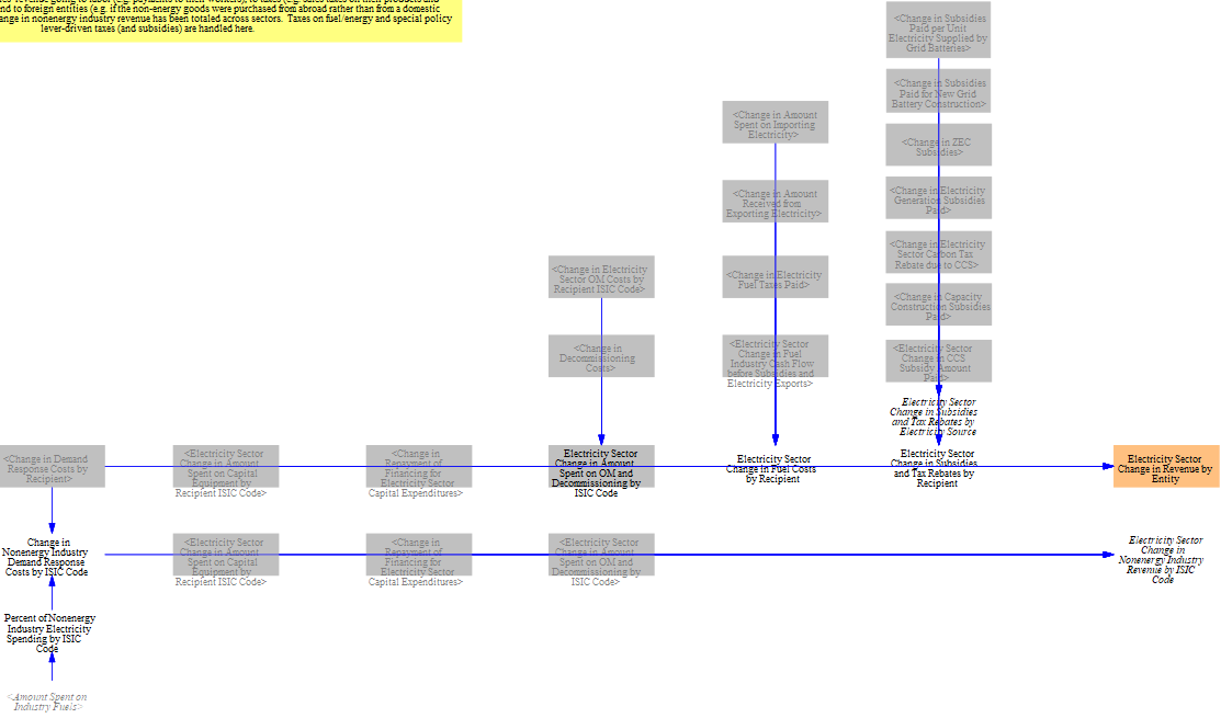
Changes in Revenue
We also need to track which entities and ISIC codes receive money based on electricity sector expenditures. To do this we sum the changes in spending by category and assign those costs to specific ISIC codes based on input data.
Changes in capacity construction costs and ongoing capital costs are aggregated and assigned to ISIC codes specific to each power plant types.
Changes in spur line costs, distribution construction costs, and transmission construction costs are aggregated and assigned to ISIC codes.
Changes in spending on batteries is assigned directly to the electrical equipment ISIC code, which includes battery suppliers.
The above changes spending are summed by ISIC code to find a subtotal of the total change in amount spent on capital by recipient ISIC code.
Changes in transmission and distribution O&M costs are aggregated and assigned to ISIC codes.
Changes in power plant fixed O&M costs are assigned to ISIC codes specific to each power plant type.
Changes in power plant variable O&M costs are assigned to ISIC codes specific to each power plant type.
Changes in CCS transportation and storage costs are assigned directly to the pipelines and transmission ISIC code.
These categories are summed to find a total change OM costs by ISIC code.
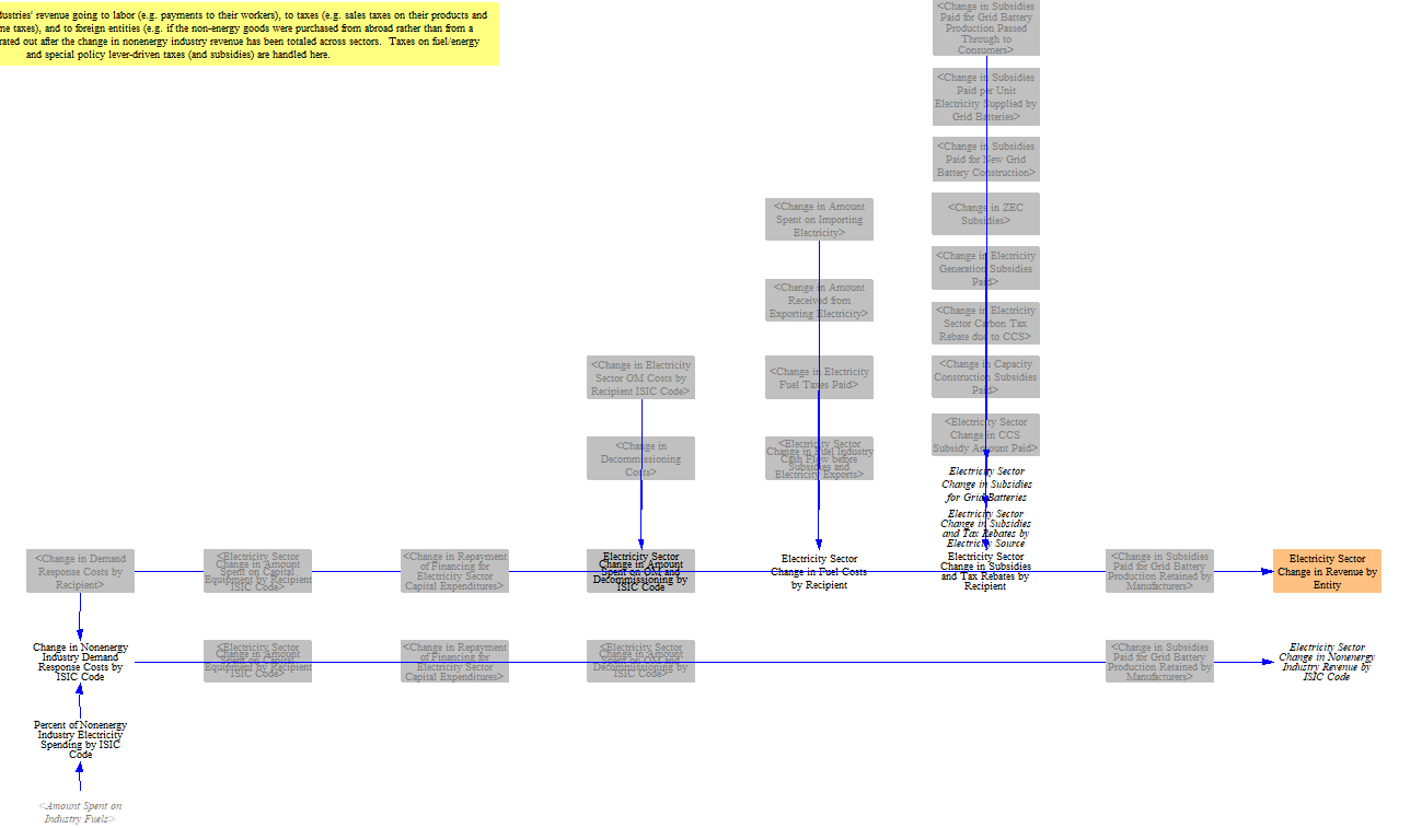
Next, we move to allocating revenues by remaining categories, e.g. decommissioning, and to allocating changes in revenues by ISIC code. Revenue from subsidies and rebates is assigned to the electricity supplier cash flow.
Revenue from fuels is assigned to the correct fuel supplier cash flow entity.
Other revenue is aggregated and assigned to the correct cash flow entity, typically covering nonenergy suppliers, such as providers of equipment used for constructing power plants.
This step also aggregates the total change in revenue by ISIC code.
Electricity Rates
The EPS estimates electricity rates, which are used throughout the model. Total rates are calculated on the Fuels page. The wholesale energy, transmission, and distribution components of the rates are calculated here in the electricity sector cash flows. The methodology is discussed below.
The model computes per-unit electricity rates along two parallel paths and then blends them. The first path is a market-based rate, in which costs that vary with the wholesale energy market and capacity market flow through to consumers via the recoverable-costs structure described in this section. The second path is a cost-of-service rate, which represents the regulated-utility framework where electricity suppliers recover the full revenue requirement (including a rate of return on rate base) directly through rates, regardless of wholesale price formation. Each path produces its own per-unit rate; the final rate seen in the model is a weighted average of the two, weighted by the share of electricity demand served under cost-of-service ratemaking versus market-based ratemaking. That share is read from input data and may differ across regions and over time. The structure described below applies to both paths; the cost-of-service path uses a parallel set of intermediate variables that aggregate the same underlying costs into a regulated-revenue-requirement framing.
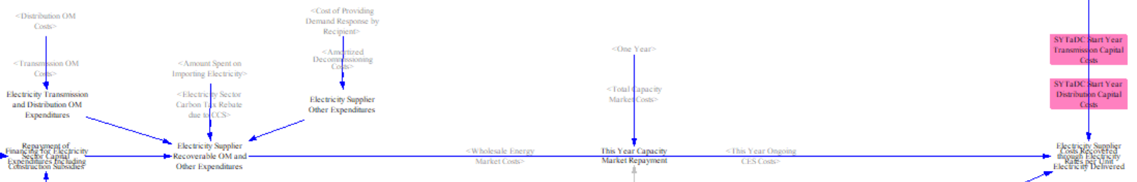
Transmission, distribution, grid storage, and battery costs are considered system costs. This means these costs, including a rate of return, are recovered directly from electricity users. These costs are treated as financed over a set financing period. To estimate the annual recoverable costs, we sum the annual change in spending for each category and apply a calculated capital recovery factor, amortizing a capital investment over an investment period and at an assumed interest rate, which is the weighted average cost of electricity sector capital specified in input data. This methodology converts annual spending by utilities into a recoverable annual cost spread out over several years. We compare these estimates to find the change in repayment for financing as well.
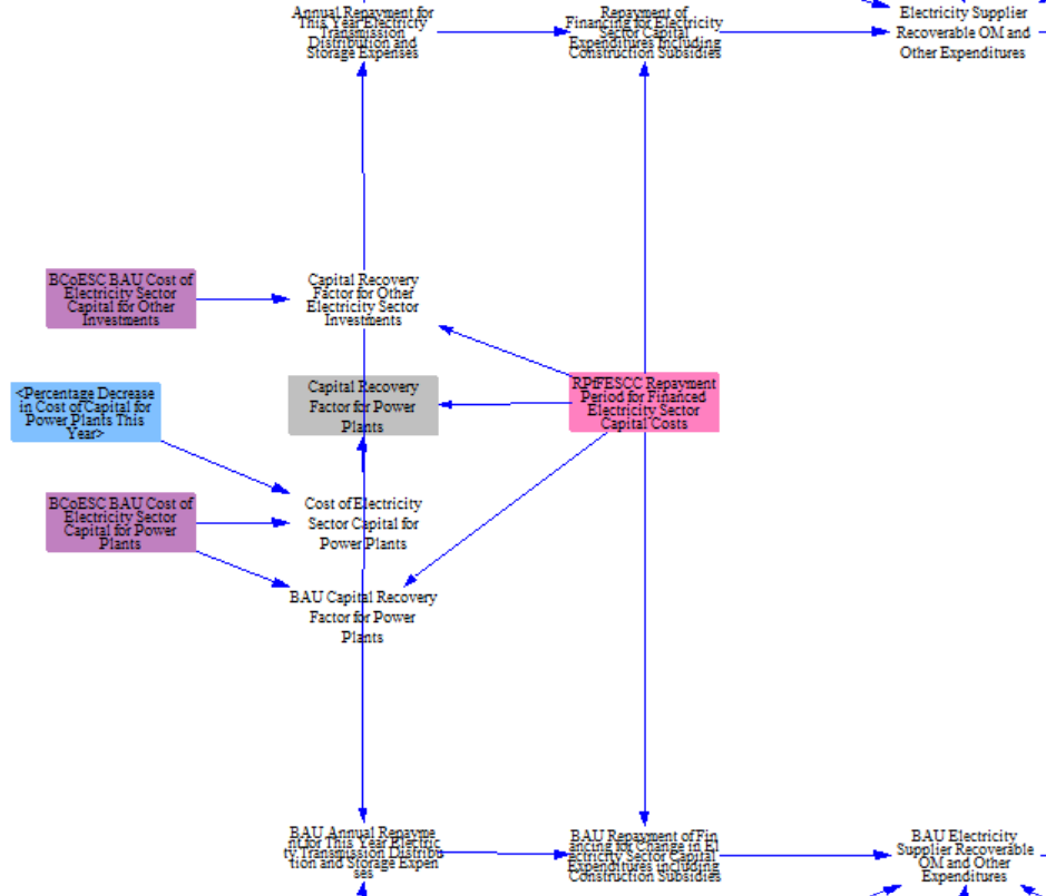
Next, we incorporate annual O&M and other expenditures. These include: transmission O&M, distribution O&M, costs of importing electricity, carbon price rebates due to CCS, costs of providing demand response, any income from subsidies paid for output from grid batteries, and the amortized decommissioning costs. All of these are considered recoverable in rates and charged directly.
Then, we move to adding other annual costs that would be recovered through rates. First is wholesale energy market costs, defined above. Next are costs of administering the capacity market or capacity construct. These costs are assumed to be folded into rates and recovered over a set period (3 years is the default), rather than all recovered in a single year.
Next, we add the annual ongoing CES costs as calculated above.
We then add in the energy costs for non-portfolio-standard-qualifying resources (i.e., resources that qualify for neither the RPS nor the CES) with zero or negative dispatch costs, also calculated above.
Summing all of the above gives us the total annual costs that need to be recovered through rates.
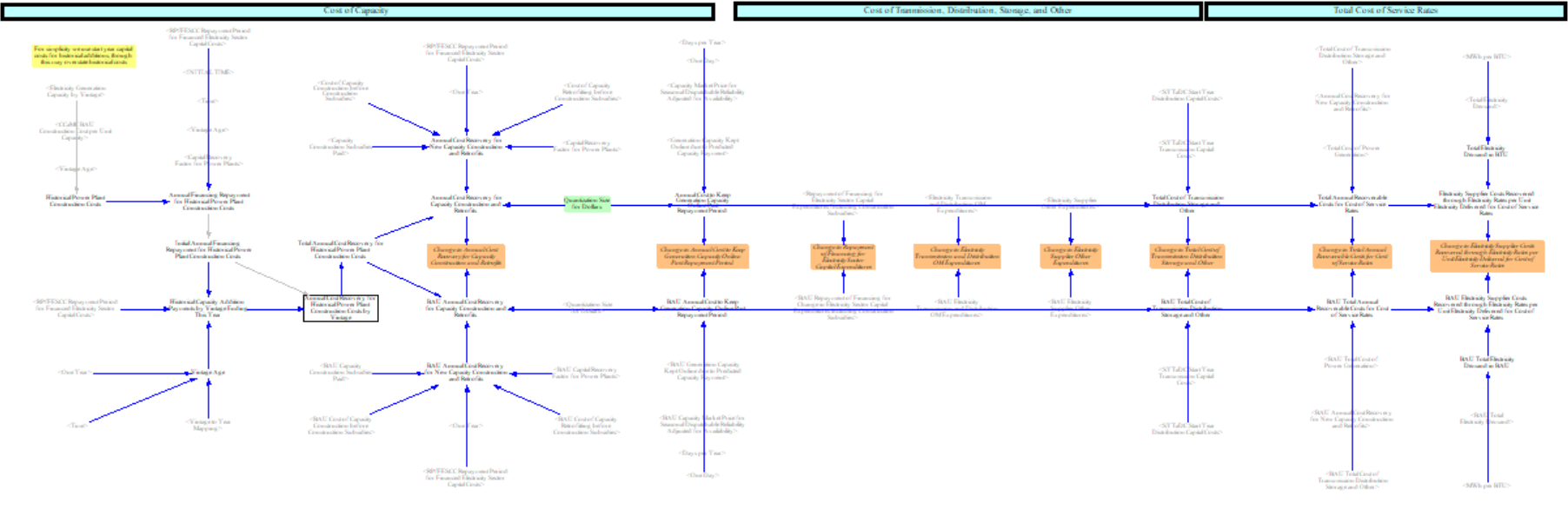
We then divide this total by the sum of total electricity demand plus exports to estimate a cost per unit electricity delivered, separately for the market-based and cost-of-service paths, and compare each against its BAU equivalent. The two are then blended using the cost-of-service share of electricity demand to produce the final rate metric.
On the fuels page, we calculate the difference between this value and cost of delivered electricity from input data, the difference of which we assume are other components of rates not captured in the model. We then calculate rates by holding this difference constant and adding it to the calculated rates using the structure above. This calculation flow is detailed on the Fuels page.
This page was last updated in version 4.0.5.