Electricity Sector (main)
General Notes
The Electricity Sector of the EPS is the most structurally complex sector in the model. In this sector, the model aggregates annual electricity demand from across the other sectors in the model, converts it to hourly electricity demand, adjusts demand based on losses, imports/exports, and load modifying technologies, and then calculates retirements, new capacity, and dispatch. Unlike other sectors of the model, the Electricity Sector has hourly temporal resolution, with the model estimating demand and generation across 24 hours in six different seasonal timeslices. It also calculates market dynamics unlike in other sectors, including the use of multiple optimization loops (iterative processes used to help a system approach a target). As such it is far more structurally detailed than other sectors.
While other sectors in the model rely on input data to specify energy or service demand, in the Electricity Sector the EPS constructs its own BAU scenario inclusive of existing policies. This different approach increases the complexity of the sector as it must be well calibrated in BAU even without the addition of policies.
The structure in the EPS attempts to mimic the behavior of other types of models that are dedicated electricity sector models, the most common of which is the "capacity expansion model." These models use linear programming to identify the least cost mix of resources that satisfy grid and policy constraints based on an objective function to minimize total system costs.
Vensim does not have the capability to use linear programming and its ability to incorporate market clearing dynamics is extremely limited. As such, we built a structure that produces similar results to capacity expansion models with a similar underlying market theory that is aligned with real world dynamics. In particular, the model will build new capacity if that capacity is profitable over a time period (meaning its anticipated revenues exceed its costs) and also if additional capacity is needed for reliability purposes, subject to a capacity price. Each component of the Electricity Sector is discussed in this section.
In general terms, the "Electricity Supply - Main" sheet determines hourly electricity demand, accounting for trade, losses, and load modifying resources. Then, it determines power plant retirements based on policy and profitability. It then runs through a series of capacity expansion steps that build new capacity, including storage capacity, based on policy, cost, or reliability, accounting for hourly demand and supply constraints. Next, it moves through a multi-stage dispatch mechanism, producing hourly dispatch and associated market prices. Lastly, it aggregates generation and calculates associated energy use and emissions. Each of these steps is explained in more detail below.
Power Plant Technologies
The model includes 24 types of power plants (note: not all of these are used in every geography the EPS covers):
- hard coal
- hard coal with CCS
- lignite
- lignite with CCS
- natural gas steam turbine
- natural gas combined cycle
- natural gas combined cycle with CCS
- natural gas peaker
- nuclear
- small modular reactor
- hydroelectric
- onshore wind
- offshore wind
- solar PV
- solar thermal
- biomass
- biomass with CCS
- geothermal
- petroleum
- crude oil
- heavy or residual fuel oil
- municipal solid waste
- hydrogen combustion turbine
- hydrogen combined cycle
In order to represent differences in characteristics between plants of the same type (say, between an older and a newer coal plant), the model uses vintaging (that is, we track when each power plant came online). Data for historical capacity is ordered by vintage and the model tracks vintages as power plants are added and retired. This allows the model to account for changes in technologies, such as improved heat rates or operating costs, over time. Generally speaking the model will order retirements from oldest to newest (more detail on retirements below). To improve runtime, the model collapses the vintages into weighted average characteristics for the fleet as far upstream as possible.
Temporal Resolution
The model includes six seasonal electricity timeslices, each with 24 hours:
- average winter day
- average spring day
- average summer day
- average fall day
- peak summer day
- peak winter day
Input data determine the number of days in each electricity timeslice. Peak days are used only in reliability calculations in the model and input data is meant to represent the worst system conditions in each hour on those days, i.e. lowest capacity factor for resources and highest demand hours. The peak hours are generally not used for computing dispatch, prices, or revenues, other than for reliability calculations.
Hourly Electricity Demand
The first stage of the power sector calculates the hourly electricity demand, which is used throughout the power sector to calculate dispatch, capacity additions, and market prices. In this stage, the model calculates the total annual demand across the various sectors and converts it to hourly demand. Then, the model adjusts hourly demand to account for trade, losses, and load modifying technologies, before finally yielding a total hourly electricity demand value for each electricity timeslice.
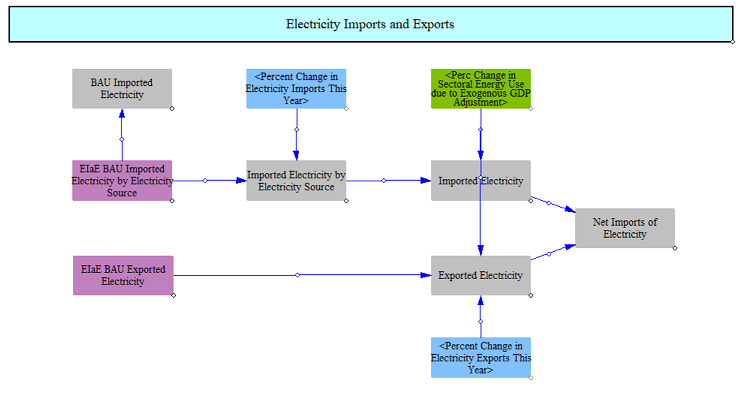
Net Imports
The EPS reads electricity exports (total) and imports (by fuel type) from input data and calculates any changes to the BAU data based on exogenous GDP adjustments determined by input data and policy levers. These adjustments vary imports and exports based on changes in GDP outside of the underlying projection data. This structure is configured to allow for estimation of COVID-induced changes in demand from data sets pre-dating 2020. The final output is total net imports (positive for imports, negative for exports).
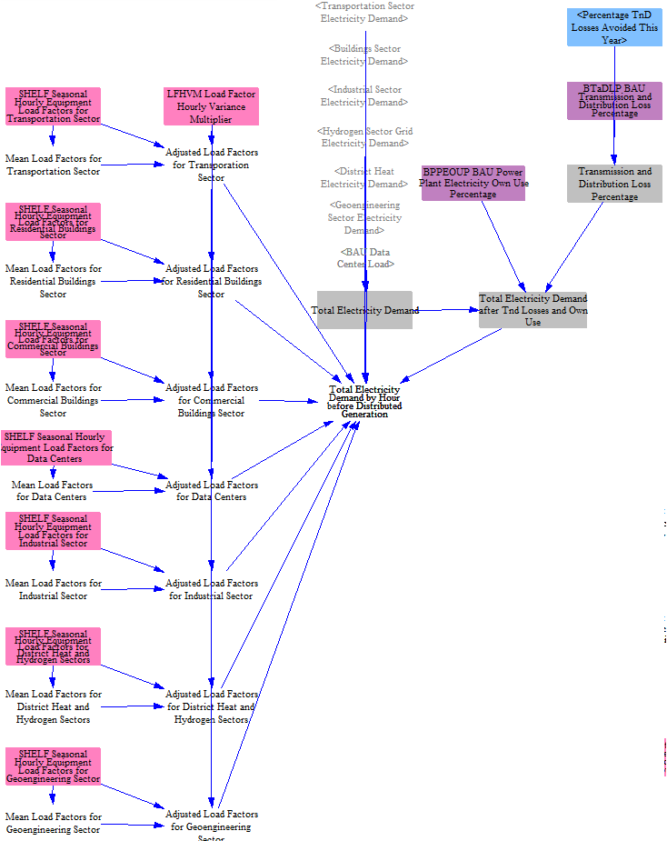
Calculating Hourly Electricity Demand from Annual Electricity Demand including Own Use and Transmission and Distribution Losses
The model then moves to compute total hourly final electricity demand. In other sectors of the model, electricity demand is tracked annually; for example, total annual cooling demand in buildings or demand for electric vehicle charging. Input data relating annual demand to hourly demand (load factors) are used to convert the annual values to hourly values aligned with the electricity timeslices used by the model.
Due to differences in data alignment, i.e. some end uses don’t directly overlap with input data, an adjustment can be necessary to ensure the computed peak and minimum demand values align with historical data. In this step, the model multiplies the computed hourly demand by an Hourly Variance Multiplier that is estimated such that the peak annual demand in the EPS aligns with historically observed values.
In this step, the model adjusts load to account for transmission and distribution losses based on input data, adding demand in each hour to cover the estimated losses. Policies can be used to improve the loss percentages as well.
Finally, the model can incorporate own use -- when some of a plant's power is used on site and never makes it to the grid -- as part of the total demand. In most regions, own use is accounted for through lower heat rates in the power sector, i.e. less power generation per unit of fuel input. But in some regions, own use is included in calculations of electricity demand, and the model can support either approach through input data modifications.
The final result is total electricity demand by hour before accounting for distributed generation.
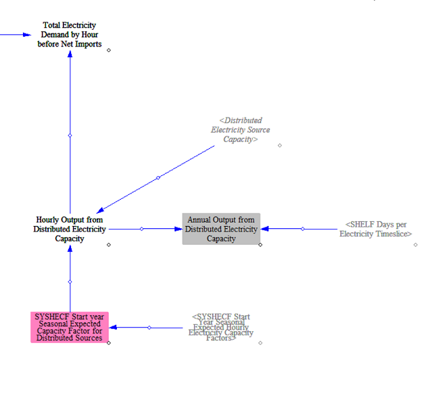
Hourly Demand after Distributed Generation
Next, the model computes the contribution of distributed resources using hourly capacity factors from input data and total installed capacity of distributed resources. Electricity supplied by distributed resources is subtracted from the total hourly demand.
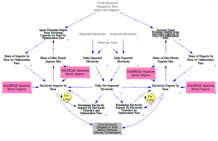
Hourly Demand after Optimizing Dispatch of Net Imports
After computing net hourly demand, the model then allocates annual net imports to hours in each timeslice. The structure proportionally allocates imports (if net imports is positive) based on the total daily share of demand in a given hour. It allocates exports (if net imports is negative) similarly, but based on the hours of least demand. Both imports and exports are subject to minimum and maximum constraints, and the model will assign all of the net imports to the next set of hours that satisfy the constraints. The model loops through 20 optimization passes to allocate imports or exports proportionally without exceeding hourly maximums and minimums, which are provided in input data.
As an example, consider a day with equal electricity demand in every hour and positive net imports. The model would allocate the same imports in every hour. Next consider a case where 23 of the 24 hours contain 70% of the daily demand, and the final hour contains 30% of the daily demand. In this case, assuming no maximum or minimum constraints, the model would apportion 30% of the expected daily import value to the worst hour and assign the remaining imports evenly across the remaining hours. Although this is a very simplified approach to estimating exports and imports, it helps maximize their utility.
Potential Load Modification from Storage, Demand Response, Pumped Hydro, and Other Load Modifying Resources
Next, the model estimates demand modifications from load modifying resources, including demand response, EV batteries, grid storage, and pumped hydro. Note that for hybrid power plants (i.e. power plants with battery storage), the impact of the onsite storage is handled through modifications to the hourly demand given limitations of programming in Vensim. This approach is discussed in more detail below where applicable.
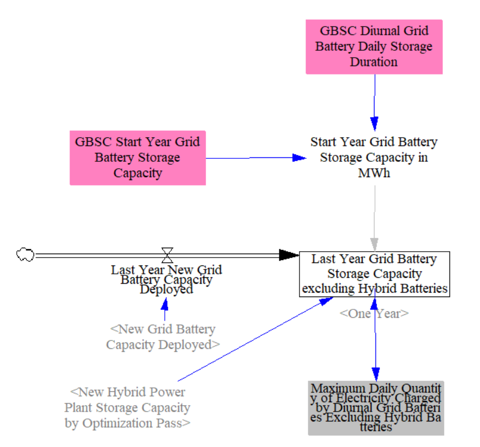
Grid Batteries Excluding Hybrid Batteries
The model estimates the total daily shifting potential of grid batteries. The model tracks the total megawatt-hours of battery capacity based on input data and calculated additions to compute a total potential. Adjustments for round trip efficiency losses are handled later in the code. The capacity additions of storage are on a one-year time delay, so the model adds the prior year's capacity additions in here. These calculations do not include the capacity of storage on hybrid power plants, which are handled later on.
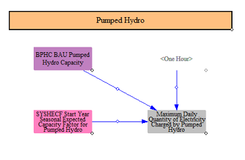
Pumped Hydro
Next the model estimates the potential day contribution of pumped hydro. Due to structural limitations in the model, pumped hydro is treated like demand response, i.e. it can be discharged daily during periods of maximum net load, and not handled as a power plant type. The model estimates daily contributions from pumped hydro by multiplying the capacity by hourly capacity factors provided in input data and assuming these rates are fixed.
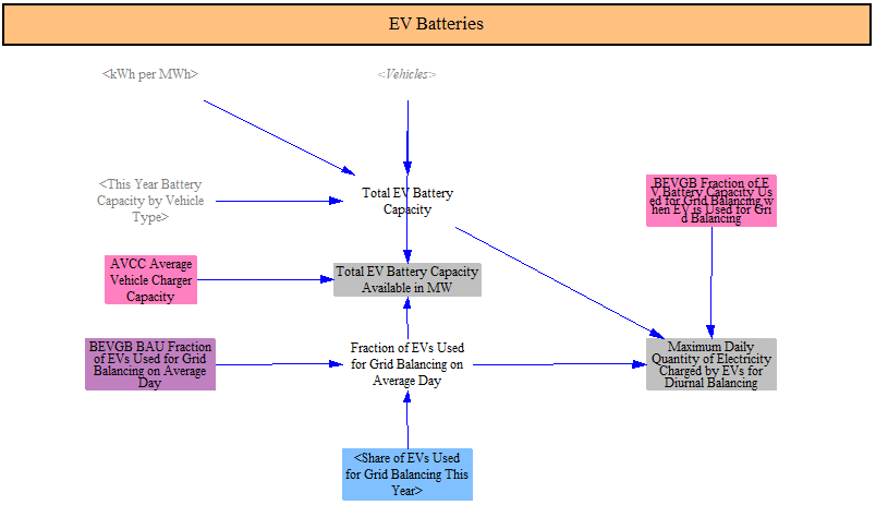
EV Batteries
EV batteries can contribute to load shifting in the EPS based on input data and policy settings. The model tracks two related but distinct measures of available EV-battery contribution to grid balancing:
- The daily energy budget (in MW·hr) that can be charged or discharged for diurnal balancing — the measure used in the load-shifting calculations described in this section. It is computed from the existing fleet's total battery energy capacity multiplied by the BAU share of EV battery capacity available for grid balancing (in many countries this is set to zero today as there is no vehicle-to-grid availability yet).
- The instantaneous power capacity (in MW) that EVs can supply to the grid as a demand-shifting resource. It is computed by multiplying the number of battery electric vehicles in each vehicle and cargo type by the average vehicle charger capacity (in kW per vehicle), summed across the fleet, and then multiplied by the same grid-balancing share. This MW figure feeds a unified
Total Demand Shifting Capacity in MWaggregator that combines EV batteries with demand response, pumped hydro, and grid + hybrid battery storage for grid-services accounting.
Users can modify the grid-balancing share through a policy lever which allows for increasing the share of total EV battery capacity that can be used for grid balancing. The model computes the final maximum amount of daily shifting that can be utilized from the EV batteries (round trip losses are accounted for later).
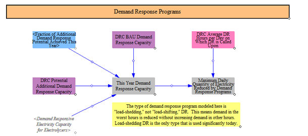
Demand Response
Total demand response (DR) capacity (in MW) is aggregated based on BAU input data and policy settings and multiplied by an average hours per day that can be called for DR to estimate the total daily contribution of DR. Note that demand response capacity is not endogenously added in the EPS. Instead, additions are specified through input data and user policy settings. The model computes a total amount of hourly load shedding by electricity timeslice that is possible from DR.
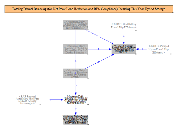
Total Diurnal Balancing Potential
The model totals the amount of load shedding and shifting available accounting for losses. Because technologies are aggregated into capacity values, the model computes a weighted average round-trip efficiency across all the different resources for use in the load shifting and shedding calculations. We also discount the availability of some resources to reflect the "copper sheet" nature of the EPS, with a power plant in one region being able to supply power in a wholly different region. Such is the limitation of a single-region model. The limiting of particular resources is incorporated via the Regional Availability Factor input file. The final outputs of this step are weighted average round trip efficiencies and total availability capacity for daily load balancing.
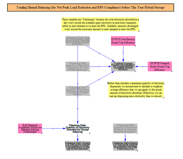
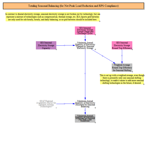
Though there are few technologies readily available, the model is structured to allow for seasonal load shifting and balancing. Input data can be configured to allow for seasonal storage capacity and to specify the annual charge and discharge cycles and round-trip efficiencies. These technologies are used later on to seasonally shift resources.
Modifying Load before Accounting for Hybrid Battery Storage
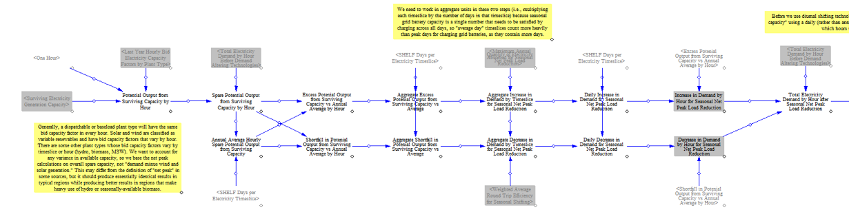
The model next builds on the calculations of load modifying resources to compute changes in load. To estimate these changes in demand, the model starts by estimating the surplus capacity in each hour. This calculation subtracts net load from available capacity in each hour, yielding surplus capacity available, which is assumed to be a good indicator of when the grid is most and least constrained. The model subtracts from this value the average for each timeslice, meaning the most constrained hours have negative values (less surplus capacity than average) and the least constrained hours have the highest positive values (more surplus capacity than average). The model then allocates net seasonal peak load reduction from the load modifying resources proportionally based on the size of the hours with less surplus capacity than average, i.e. the hours with the least surplus capacity have the highest net peak load reduction from load modifying resources. For storage resources, charging hours are proportionally allocated to those hours with the most surplus capacity, accounting for round trip efficiency losses.
After calculating the seasonal load shifting, the model then calculates diurnal load shifting and shedding based on the resource availability calculated earlier. The model then aggregates the total load shedding and shifting across seasonal and diurnal resources and computes a total amount of hourly electricity demand after demand altering technologies.
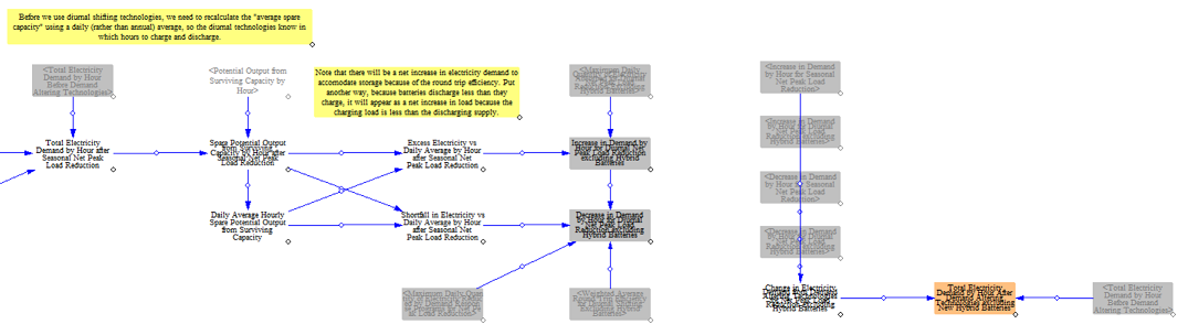
Modifying Load after Accounting for Hybrid Battery Storage
The model next passes through another round of load modification using the adjusted load as a starting point. This part of the model also integrates with the capacity expansion structure to optimize the deployment of hybrid storage resources (i.e. wind and solar with storage) based on when they would charge and discharge and modifies the load accordingly. This approach is somewhat unique in that it modifies load to reflect charging and discharging of hybrid resources given constraints in the structure of Vensim. This step of the model is co-optimized with hybrid power plant capacity expansion so that the capacity and load impact is optimized.
First, the model calculates an updated amount of battery storage for load shifting inclusive of hybrid batteries. The model does this in 20 optimization passes which are synced with capacity additions and in each pass further refines the storage capacity based on the calculated storage additions in the current pass.
The model follows the same approach as before, moving through load modification from seasonal storage and diurnal storage, but using the values calculated in the first load modification pass for resources other than battery storage.
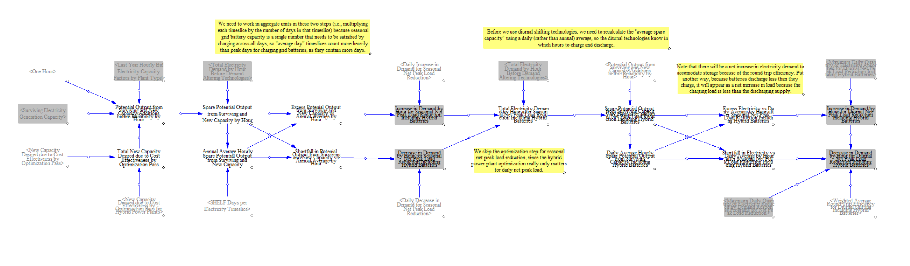
The model incorporates the new load shifting amounts into demand and produces final hourly electricity demand using the storage additions from the final optimization pass.
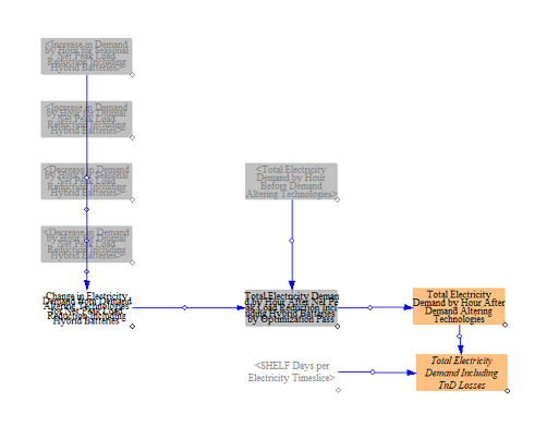
At the end of this calculation flow, the model has determined the final hourly electricity demand that must be met by generation resources and accounts for all load reduction and shifting that occurs from distributed resources, imports and exports, load modifying resources, and hybrid power plants.
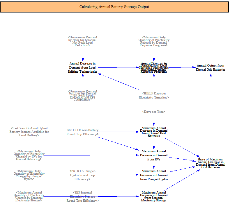
Summing Charging and Discharging from Batteries
The model sums the total amount of battery capacity and the total charging and discharging of batteries, inclusive of hybrid batteries, for use in other places throughout the model. For hybrid batteries (those paired with a renewable resource at the same plant), the model decides which hours to charge and discharge by treating the previous five-year average marginal dispatch cost as a price signal: a Vensim allocation function distributes each day's charging budget toward the hours with the lowest prices and the discharging budget toward the hours with the highest prices, so that hybrid storage tends to charge when cheap power is plentiful and discharge when prices are high. Standalone grid batteries continue to use the load-shifting allocation mechanism described in the diurnal-balancing sections above.
Revenues, Costs, Retirements, and Max Build Rates
This stage of the model calculates revenues for new and existing resources, uses this information to estimate retirements, and calculates maximum build rates based on technical potential for different resources.
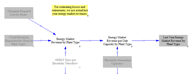
Annual Energy Market Revenues for Existing Resources
To estimate energy market revenues for existing resources, the model calculates total revenue per unit capacity by summing the hourly generation from all resources of a certain type (e.g. natural gas combined cycle power plants) and the marginal dispatch cost in that hour and dividing by total installed capacity, yielding estimated annual energy market revenue per unit capacity.
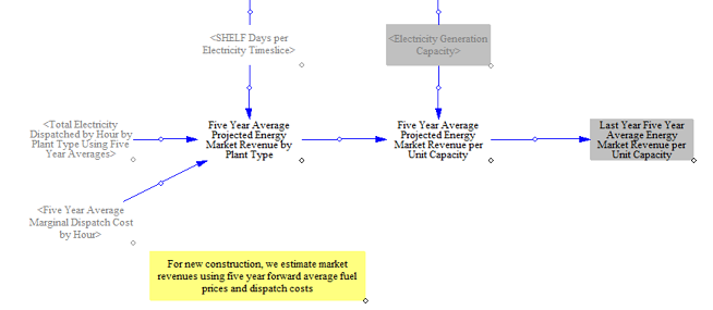
Projected Annual Revenues for New Resources
For new resources, the model estimates potential energy market revenues for plants with and without existing capacity. For plants with existing capacity, the model estimates potential dispatch and energy market revenues use a five-year average of energy prices for various resources, in order to average out annual fluctuations in resource costs.
For plants without existing capacity, the model calculates a hypothetical dispatch amount in each hour as if that resource had been available using the calculated hourly energy market prices for existing resources (discussed later). This allows us to estimate potential dispatch and revenue from plant types with no existing capacity in the model but which may become profitable and be built in later years, such as hydrogen-based plants.
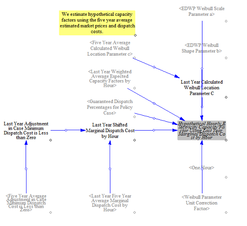
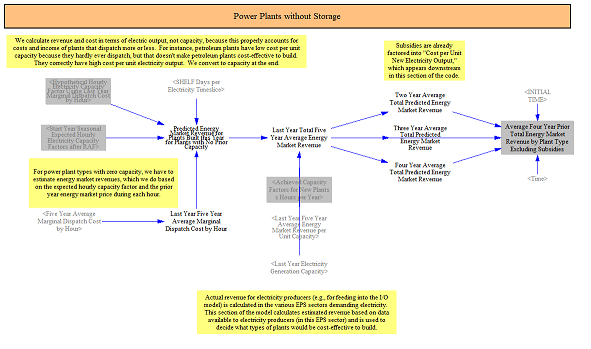
The model combines the hypothetical dispatch for new resources with no existing capacity and the five-year average marginal dispatch costs to produce estimated annual energy market revenues for planning new capacity. This is combined with the five-year estimated energy market revenues for resources with existing capacity to produce a value for all new resources. Costs are divided by expected capacity factors to levelize them into a $/megawatt-hour value for all plant types.
Given the structure of the EPS and that it calculates load dynamically, it does not have foresight. To make future planning decisions in the electricity sector, the model therefore relies on a rolling average of energy market revenue. The model calculates a rolling four-year average of anticipated energy market revenue (using five-year averages for fuel prices as outlined above) for guiding investment decisions. In the first several years of the model run, prior to enough years being run to produce a four year average, the model will use the highest number of years possible to create the average, i.e. one in year one, two in year two, three in year three, and four in all subsequent years.
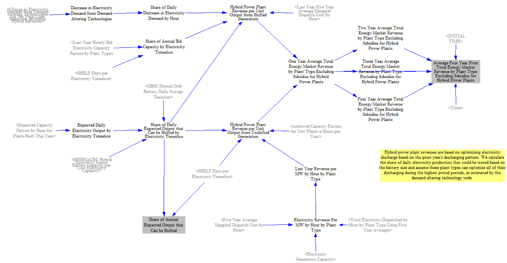
The model has to calculate projected energy market revenues for hybrid power plants separately because they are able to optimize discharging and charging of the battery to maximize energy market revenues. To calculate the revenues the model applies input data on the average battery capacity per unit power plant capacity to compute the storage amount per MW of power plant capacity. It then calculates the share of daily expected output that can be shifted, which varies across electricity timeslice because of varying capacity factors by timeslice. The model computes the revenue from shifted generation based on availability and battery size and adds to it the revenue from unshifted generation to compute a total levelized energy revenue per unit output. This value will be higher than for plants without storage, particularly when there is a significant spread in marginal dispatch costs. These revenues also use the five-year fuel price averaging outlined above.
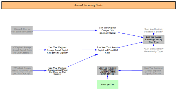
Annual Recurring Costs
Annual recurring costs are calculated as an input into the retirement decision-making framework. These costs are the sum of dispatch costs (which include fuel and variable O&M), annual capital costs (from input data) needed to maintain plants' operability, and ongoing fixed O&M costs. The model computes these costs on a $/MW basis for use downstream in retirement calculations
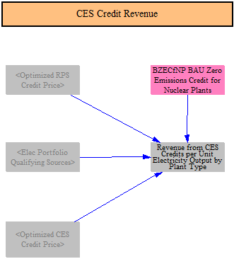
Clean Electricity Standard and Zero Emission Credit Revenue
Input data can specify any credits specifically for nuclear power plant owners. The model calculates credit prices from the clean electricity portfolio standard (discussed later) which are used here. The portfolio standard is represented as a unified framework that can simultaneously enforce a Renewable Portfolio Standard (RPS) and a Clean Energy Standard (CES) -- the two are configured independently with their own qualifying-resource definitions and percentage targets, and a separate credit price is computed for each. Total revenue from these credits, summed across the RPS and CES paths, is calculated for use in the retirement calculations.
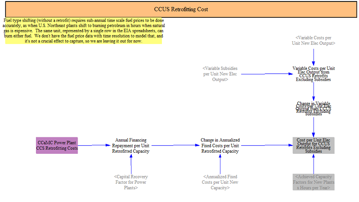
CCUS Retrofitting Costs
CCUS retrofitting costs are calculated using estimated capital costs and a capital recovery factor (an estimate of how much a borrower needs to pay each year to fully recover the cost of an investment and accrued interest), and incremental variable and fixed O&M costs from converting to CCUS. This yields an estimated retrofitting cost per unit electricity output. CCUS plants can have higher capacity factors than non-CCUS equipped plants, which can contribute to lowering the incremental cost difference.
Annualized Cost per Unit Output for New Capacity (i.e. LCOE)
Annualized costs per unit new electricity output, the EPS version of an Levelized Cost of Energy (LCOE), is calculated next. These costs start with capital costs based on input data and endogenous learning of capital costs for certain technologies. The model starts by splitting soft costs and hard costs and applying an endogenous learning rate to the capital cost portion where that structure is used (discussed in the endogenous learning section of model documentation). Policies can be used to further lower soft costs. Research and development policies can also be used to further lower the total construction costs (sum of hard and soft costs).
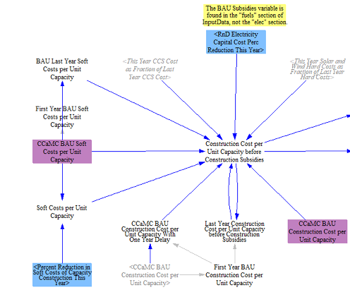
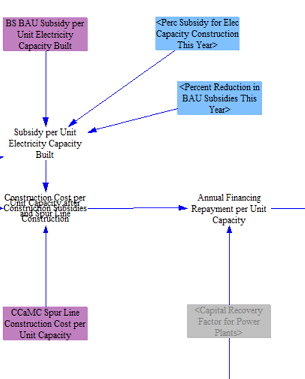
The model then applies any subsidies for capacity construction (e.g. investment tax credit), which can be modified by user set policies. The model also adds in spur line costs at this point, which vary by technology and region. After computing the construction cost after subsidies and spur line costs, the model estimates an annual repayment of these costs per MW using a capital recovery factor calculated upstream. Each plant type can have its own capital recovery factor which is based on the weighted average cost of capital and assumed financing lifetimes for power plant types. The application of the capital recovery factor converts the construction costs into an annualized payment.
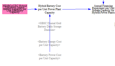
For hybrid power plants, the model calculates the incremental annualized financing payment from the additional storage at the power plant.
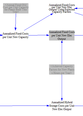
Next, the model adds annual fixed operating and maintenance (O&M) costs to the annualized financing repayment, then converts the annualized costs to levelized costs based on the achieved capacity factors of various types, yielding a $/Megawatt-hour value for all plant types. The anticipated capacity factors utilize historical three-year data calculated in the model to adjust capacity factors as the grid evolves, i.e. if natural gas combined cycle units dispatch less because there is more clean electricity on the system, the capacity factors reflect this evolution, and the levelized costs increase.
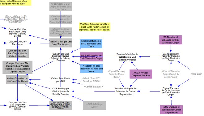
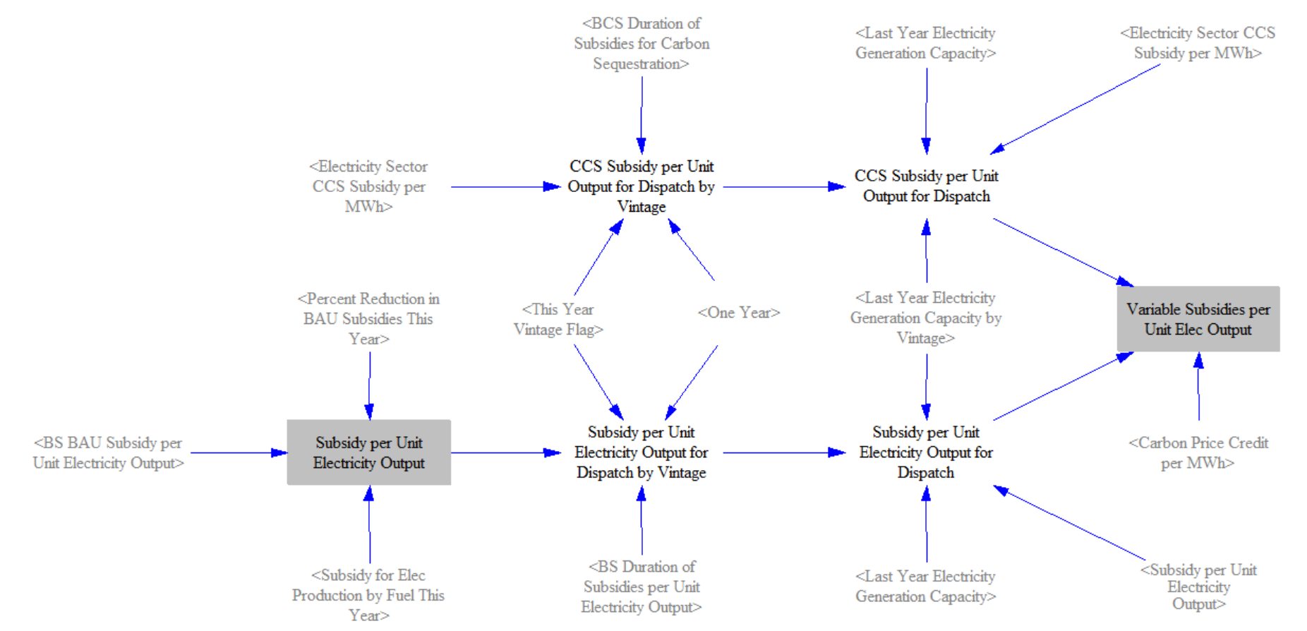
The model then estimates total variable costs and subsidies. Electricity production CCUS subsidy amounts are calculated here, including an adjustment based on the lifetime of the credit (i.e. for credits that are only available for a portion of the financial lifetime of the power plant, their value has to be adjusted to account for the limited duration of their availability). The model adjusts the value of the incentive to account for instances where the duration of the subsidy is shorter than the financial lifetime of the plant (i.e., what is the value of a 10-year subsidy on a plant lasting 20 years). Users can also modify the electricity production and CCUS incentives, which change the subsidy per unit electricity output. Carbon pricing credits are also calculated at this stage for plants equipped with CCUS. The model sums total variable costs, including fuel costs (which include carbon pricing impacts), variable O&M costs, CO2 transport and storage costs per Megawatt-hour for plants with CCUS, electricity production subsidies, carbon price credits, and CCUS subsidies. Variable costs are added to the levelized fixed costs to produce a total cost per unit new elec output and several variations on this variable used throughout the model. Storage costs are added to these values for hybrid power plants.
Economic, Policy-Driven, and Planned Retirements
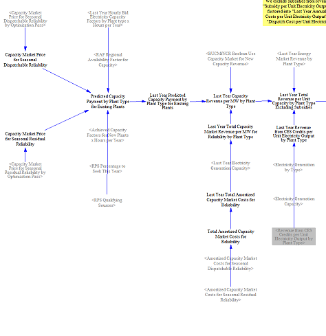
The model next moves on to calculating total annual retirements. Total revenues are calculated, including capacity market revenue or capacity contract revenue (discussed later), energy market revenue, revenue from clean electricity credits, and revenue from zero emissions credits, yielding a total revenue per unit capacity.
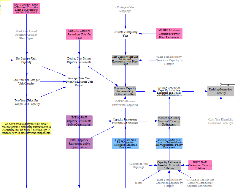
For each power plant type, annual revenues are compared against going forward costs, calculated earlier, to estimate a net loss per unit electricity capacity. Power plants must be uneconomic (have net losses) for at least three consecutive years to be deemed uneconomic. If there are net losses for at least three years, the model calculates the rolling average three-year net loss and multiplies this by a calibrated parameter to determine the total cost driven retirements in a given year.
To this, the model adds capacity retirements specified in input data and finally adds capacity retirements from any policy lever settings to determine total retiring generation capacity.
The model also supports a third, optional retirement path based on a fixed economic lifetime per power plant type. When this path is enabled (via a control setting), the model retires capacity in the year that its vintage age equals the configured economic lifetime for its source type, in addition to any economic and policy-driven retirements that would otherwise occur. This complements the economic retirement mechanism described above and is useful for calibration and for representing plants that are scheduled to retire at expected end-of-life regardless of profitability. The control setting is off by default in the U.S. model.
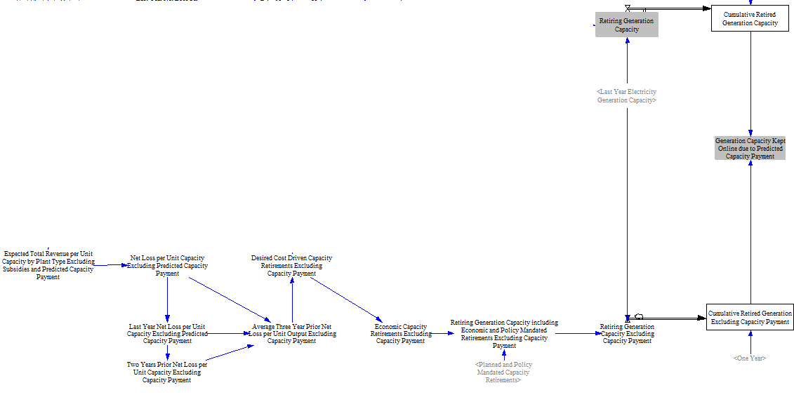
We duplicate this structure below but exclude plants' predicted capacity market revenue. The retirements calculated here are not used in the calculation flow; rather the difference between modeled cumulative retiring capacity and the value without capacity payments is used later in the cash flows to estimate system capacity costs.
Maximum Buildable Capacity
The model accounts for technical potential for various power plant types and will not allow capacity to be built in excess of maximum technical potential, particularly for renewable resources. In addition, policy levers can be used to restrict the construction of certain capacity types. If a power plant type has been fully retired from the model, it is not allowed to be built again in later years. Collectively these calculations yield a maximum capacity buildable in a given year. The model includes other annual restrictions for new capacity, which are discussed below in the section on new capacity construction.
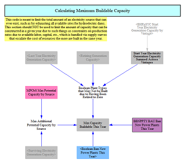
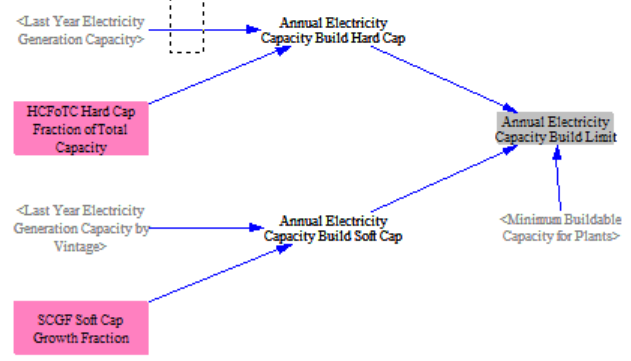
The model also limits how quickly each source's capacity can grow from year to year, reflecting real-world supply-chain and deployment constraints. Each source is subject to an annual build limit equal to the smaller of two caps: a soft cap, equal to the largest single existing vintage of that source's capacity grown by a configurable growth fraction, and a hard cap, equal to a configurable fraction of total system capacity. The annual build limit is the lesser of these two, but never less than a minimum buildable amount, so that small or nascent technologies can still be deployed. Both the growth fraction and the hard-cap fraction are set in input data.
New Capacity Construction
In this stage, the model calculates new capacity additions across multiple mechanisms. The first of these is a mandated capacity and retrofit mechanism that uses input data and policy levers to add capacity and retrofit plants with CCUS. Next the model will add clean firm capacity if needed to comply with a clean electricity standard. After this step, the model moves into adding economic capacity, which is co-optimized with the clean electricity standard policy. Lastly, the model moves through a two stage reliability capacity addition mechanism, which ensures there is sufficient capacity installed to meet reliability requirements.
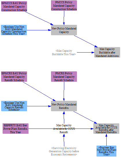
Policy Mandated Capacity Additions and Retrofits
Mandated capacity additions and CCUS retrofits in the BAU and policy scenarios can be specified in the input data and policy levers. The model starts by reading in these values and adding them to new capacity built and retrofits in future years. The model maintains two independent mandate paths: a per-electricity-source generation mandate (covering the 24 generation technologies listed above) and a grid-battery storage mandate, each with its own BAU input schedule and its own non-BAU policy lever. The grid-battery path uses BPMGBSA BAU Policy Mandated Grid Battery Storage Additions as its BAU input. The two paths are independent, so a user can override mandated grid-battery additions without disturbing mandated generation construction, and vice versa.
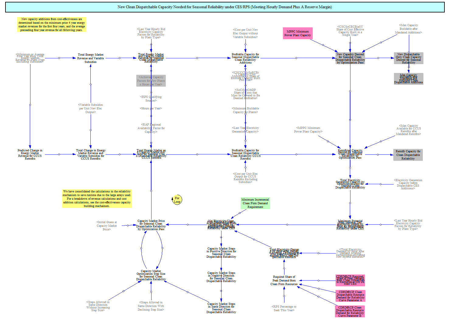
Flexible Clean Capacity Additions and Retrofits Required for Clean Electricity Standard Compliance
Next, the model calculates whether or not new clean dispatchable resources are needed to meet the clean electricity standard and will build new clean resources or retrofit existing ones if capacity is needed. We use a simplified assumption that 5% of peak demand at a 100% clean electricity standard value must be met with clean dispatchable resources in order to ensure the model builds sufficient clean dispatchable resources given its other constraints. In years leading up to the 100% clean electricity standard, the annual amount of clean dispatchable capacity required is determined by an s-curve defined in input data.
Each capacity mechanism, excluding mandated additions, uses a structure that computes the cost-effectiveness of resources and determines the amount to be built if they are cost-effective. This structure is covered in more detail in the next section.
If new clean dispatchable capacity is needed that would not otherwise be built, the model computes a credit price for new resources that drives sufficient new capacity to meet the demand. The model will increase the credit price until sufficient resources are built, based on the total revenue of various technologies, to meet the requirement. It adds this revenue to the estimated revenue for different plant types and then computes the amount of capacity added. The cost of this credit is added to the total costs of the clean electricity standard program.
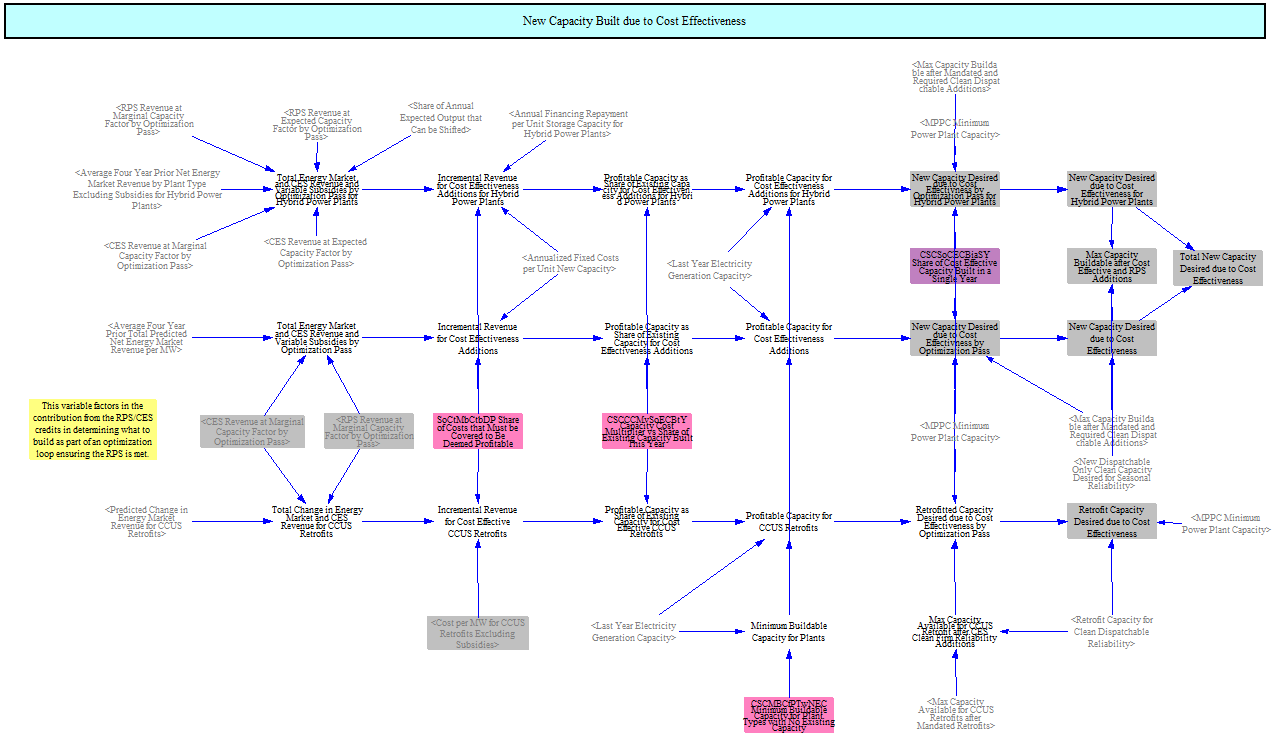
Cost Effectiveness Additions and Retrofits
The core logic underpinning each element of the capacity expansion structure operates by evaluating whether power plant types are profitable and estimating additions based on their level of profitability. Policies can affect this profitability through adding revenue to specific power plant types.
This mechanism operates simultaneously for new resources without storage, new resources with storage, and CCUS retrofits of existing resources.
The model begins by cumulating the total anticipated revenue by resource type. This relies on the rolling four-year energy market revenue discussed earlier and any anticipated policy revenue, particularly credits from the portfolio-standard mechanism (RPS, CES, or both), which is co-optimized with economic capacity expansion (discussed later). Revenue is normalized into $/Megawatt-hour based on achieved capacity factors by resource in the model. Subsidies for electricity generation are added.
The model then compares anticipated revenue against the anticipated levelized cost of building new resources, not including variable subsidies (these are considered a revenue stream). Resources that are profitable will have revenues that exceed costs while unprofitable resources will not. This results in a profit value, i.e. revenues minus costs.
The model then plots the expected profit against a curve that is defined in input data and calibrated against historical data and other models. The curve plots profit against a share of existing capacity, translating the profit amount to a share of existing capacity. This curve defines how much capacity is built for a given profit margin based on the total installed capacity of each resource. This prevents the model from overbuilding novel resources and lets the model deploy incremental capacity at a given profit level as the total installed capacity of that resource grows and the knowledge, labor force, and materials become more widely available
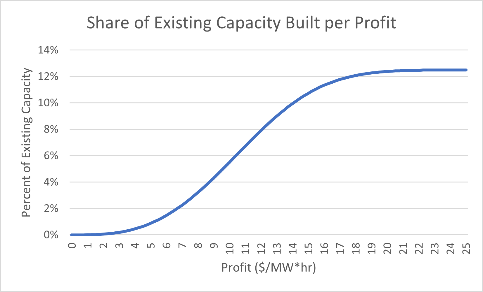
For example, if a resource type has a profit of $10/Megawatt-hour, it would cause new builds of roughly 5% of existing capacity. For a resource with an installed base of 50 GW, this would yield 2.5 GW of new builds. But over time as more of that resource is built, if it gets to 100 GW, then the same profit level would result in 5 GW being built. (This is balanced in the model by evolving market revenue as the system is saturated with resources).
The model then computes the total new capacity added using this computed value and several input data files which let users change the share of costs that have to be covered to be deemed profitable and the share of cost-effective capacity that is actually built (sometimes there are market dynamics that significantly limit what can be built, even if it is profitable) The model also uses a minimum value for resources that do not yet exist so that it is always capable of building them if they are profitable.
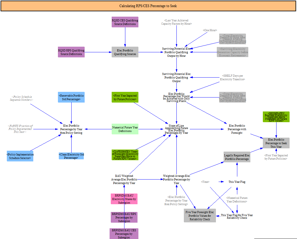
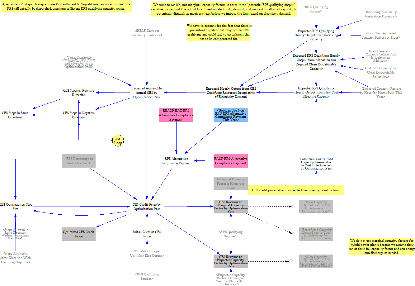
Clean Electricity Standard Additions
The EPS represents electricity portfolio standards through a unified framework that can simultaneously enforce a Renewable Portfolio Standard (RPS) and a Clean Energy Standard (CES). RPS typically qualifies only renewable resources (wind, solar, geothermal, hydro, etc.); CES is broader and may also qualify nuclear, fossil generation paired with carbon capture, and other low-carbon firm resources. The model treats the two as configurations of the same machinery: each has its own qualifying-resource definitions, its own percentage targets (which can also vary by subregion), and its own credit price that the model converges on. A run can enforce either standard, both at once, or neither. Where these docs below use the abbreviation "CES/RPS," it refers to whichever of the two standards is being computed in that step.
The application of each portfolio standard is co-optimized with the cost-effectiveness additions to identify a credit price that generates sufficient revenue to add or retrofit resources for cost-effectiveness that leads to compliance with the standard. In each optimization pass, the model checks to see whether the anticipated amount of existing and new or retrofit qualifying electricity is sufficient to meet the target. It will raise the credit price until this share is met and converge on a credit price that gets just the right amount of new qualifying capacity built and/or retrofit. The RPS and CES optimizations run in separate passes, so each finds its own marginal-clearing credit price.
The first stage is to compute the weighted average national CES/RPS value. The model allows for different resources to be included as part of the RPS or CES and aggregates subnational data provided in the input data to estimate a binding value. For example, many states have existing RPS/CES values and collectively they form a national floor, below which a user policy setting would not be binding. This first set of structures computes the effective RPS/CES value that the model will achieve, separately for each. In parallel, the model optionally determines the portfolio percentage needed to meet future RPS/CES values if foresight is enabled.
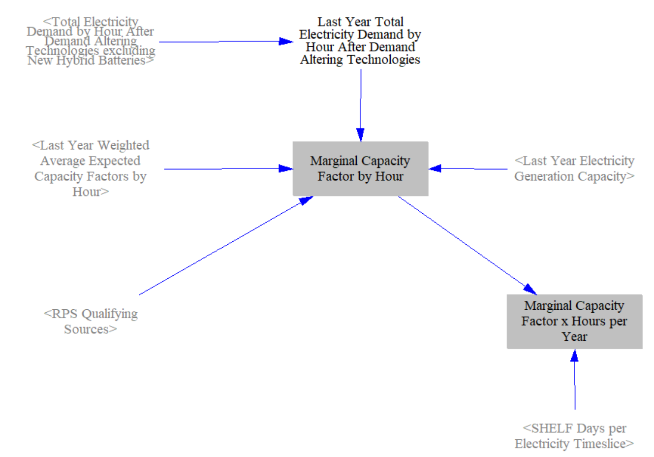
The optimization structure utilizes a special type of capacity factor, the marginal capacity factor, in order to properly incent and build the right resources. This is needed because once certain hours are saturated with clean electricity, adding more clean electricity in those hours does not help increase the total share of clean electricity over the year. The marginal capacity factor captures the diminishing value of resources as the grid gets cleaner and certain hours are saturated by variable renewable sources.
One drawback to this approach is that it can make the credit price seem unnecessarily high. This can occur because the model computes revenue as the CES credit price multiplied by the marginal capacity factor for a given hour, summed over the year. As the grid approaches 100% clean, marginal capacity factors for all resources decrease and a higher price is needed to drive clean adoption. On the other hand, this ensures the model is only paying for completely additive clean resources and it helps shift CES revenue to dispatchable resources as the grid gets close to 100% clean.
Hybrid resources are included in the optimization loop and the model will tend to move towards them in years with higher clean shares to reallocate the clean supply to the hours when it is needed. Because a hybrid resource (a renewable paired with on-site storage) can be desired both as a hybrid power plant and as a standalone generation source, when the combined desired additions for both roles would exceed what is buildable for that source, the model splits the buildable capacity between the two roles in proportion to each role's desired amount as a proxy for comparative profitability.
The CES also allows users to set an Alternative Compliance Payment in the input data that sets a cap on the credit price. Once the cap is hit, the model will not continue to increase the credit price, even if it cannot hit the CES target. Relatedly, when a portfolio target cannot be met even with full deployment of qualifying resources — that is, the maximum achievable clean share is at or below the target — the model detects this during the optimization passes and holds the final credit price at the level that achieves the maximum feasible buildout, rather than continuing to step it upward.
The CES optimization works together with the clean dispatchable mechanism so that the model doesn’t overbuild clean resources but builds adequate flexible clean resources.
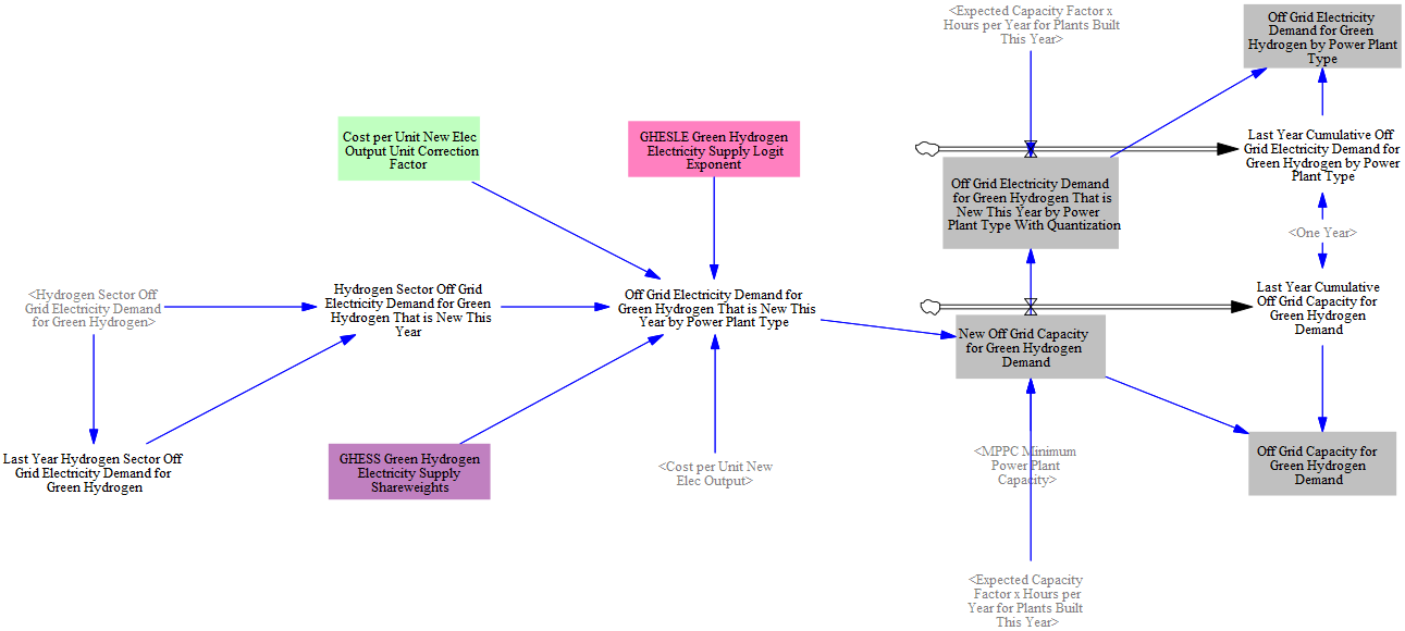
Additions to Support Green Hydrogen Production
The EPS also tracks green hydrogen demand and will build off-grid renewables to support the production of green hydrogen. This part of the model uses a logit choice function to assign the demand for electricity to different resource types based on their costs. The exponents and shareweights for logit are included as part of input data. The model then builds sufficient capacity to electricity demand for green hydrogen production and tracks this stock over time.
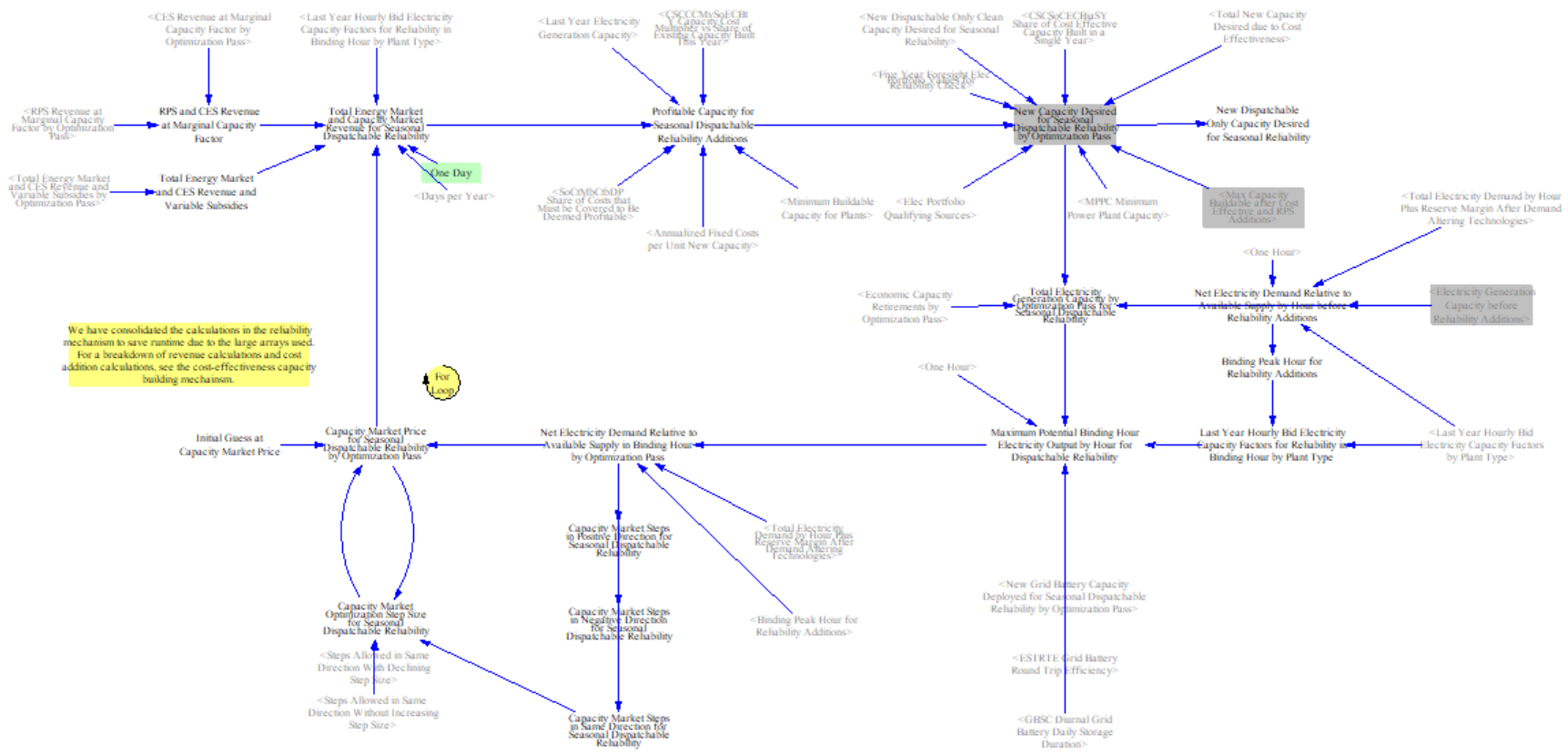
Reliability Additions
At this point the model has built capacity as mandated in input data, for cost-effectiveness, to comply with an RPS or CES including if flexible clean resources are needed, and for off-grid green hydrogen production. The final capacity mechanism ensures there are sufficient resources online to meet reliability in every hour, including a reserve margin.
In practice, reliability additions in the EPS comprise dispatchable resources -- the kinds of plants utilities and grid operators rely on to provide firm capacity during peak demand hours (e.g., natural gas peakers, nuclear, hydro, biomass, dispatchable storage). Variable renewable resources like solar PV and onshore wind do not effectively enter through this mechanism because their availability in the binding peak hour (typically a winter evening for many regions, when solar output is zero) is very low; the capacity-market revenue they would receive in this calculation is discounted by that availability and is too small to make them profitable for reliability additions. They enter the model instead through the cost-effectiveness, portfolio-standard, and policy-mandate mechanisms above. This restriction reflects real-world capacity planning practice, where reliability is provided by firm and dispatchable resources rather than by variable renewables.
To size additions, the model first identifies the single binding peak hour -- the (timeslice, hour) combination across the peak winter and peak summer days where net electricity demand most exceeds the available supply, after accounting for the reserve margin. It then computes a capacity price that increases revenue such that sufficient dispatchable capacity is added to the system, using the same cost-effectiveness structure used elsewhere in the model. Resources' total revenue from the capacity price is discounted by their hourly availability in the binding hour. For example, if a winter 10 PM peak is the binding hour, dispatchable resources receive capacity revenue weighted by their typical availability in that hour.
To estimate how much is needed in each hour, the model uses a peak winter and a peak summer timeslice. These are meant to represent the worst system conditions during the worst days of each season in terms of demand and potential output from variable resources. The input data uses hierarchical clustering of historical demand data and the minimum capacity factor for variable resources. The model then adds a reserve margin to ensure sufficient supply. These approaches attempt to mimic planning procedures of real-world utilities and grid operators.
The reliability mechanism runs two parallel sub-computations on disjoint subsets of dispatchable resources, both summed into a single set of reliability additions:
- Clean dispatchable reliability -- restricted to dispatchable resources that qualify under the active CES (e.g., nuclear, hydro, geothermal, biomass with CCS, gas with CCS). This sub-pass ensures that as a CES approaches 100%, the model can still maintain reliability with qualifying resources rather than non-qualifying generation.
- General dispatchable reliability -- the remaining dispatchable resources (e.g., natural gas peakers in regions where the CES does not require carbon capture). This sub-pass handles reliability needs that don't have to come from CES-qualifying resources.
Both sub-passes use the same binding-peak-hour structure described above. Their resulting capacity additions are summed and added to the generation-capacity total going into stock-and-flow tracking.
Because the reliability mechanism runs downstream of the cost-effectiveness mechanism, including for the CES/RPS, it can result in additional dispatchable clean capacity being built that pushes the model past the CES/RPS target in certain years. The only way to fully avoid this would be through a linear program where the model could optimize capacity against multiple constraints at once, but Vensim is unable to do this.
If the model has a CES/RPS of 100%, the reliability mechanism will not allow non-qualifying resources to be built. However, in the years leading up to the 100% value, the model can still build non-qualifying resources, which may not be run or may not be allowed to run shortly after. This is a known issue using a model without perfect foresight, but we are again constrained by our ability to model this given Vensim’s structure. A future area for enhancement might be to integrate the future year RPS value into the reliability structure to prevent the model from building resources that would never or only scarcely be used.
Total New and Retrofit Capacity
Lastly, the model sums the total capacity additions and retrofits for input into the stock and flow tracking.
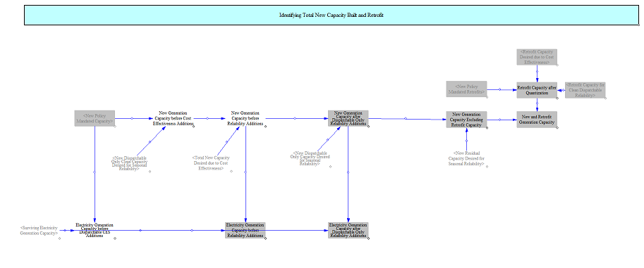
Tracking Electricity Stock and Average Power Plant Fleet Properties
This part of the model tracks fleetwide properties of power plants, such as installed capacity, weighted average heat rates, and operating costs. The model collapses the vintaging here into a single weighted average value to minimize runtime impacts and carry through a single value for each power plant type.
Tracking the Electricity Fleet
Existing capacity, retirements, new capacity, and retrofits are combined to produce key outputs for use across the electricity sector.
![]()
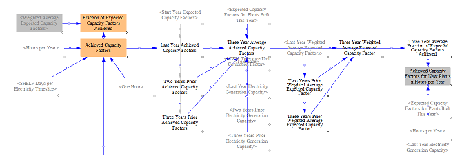
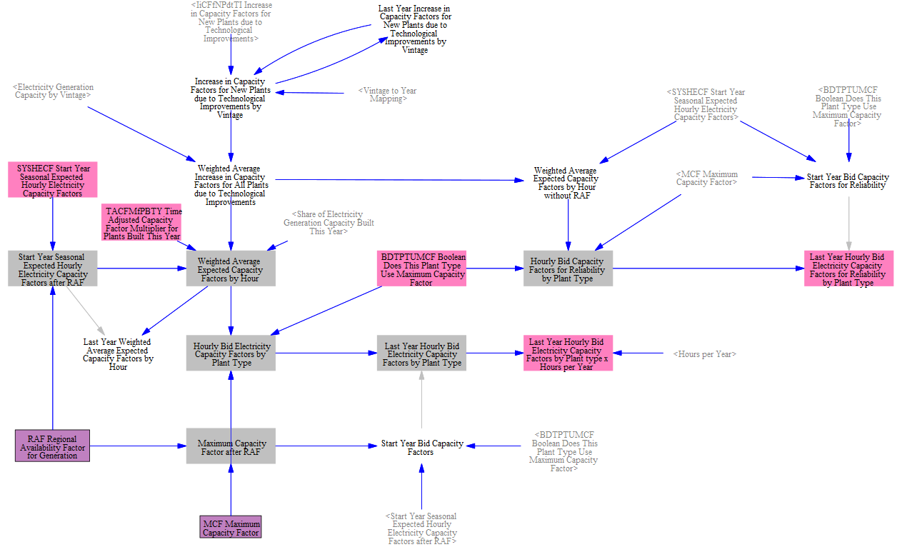
Capacity Factors
Various capacity factor calculations are used through the electricity sector. These include achieved capacity factors (annual and by hour), three year average achieved capacity factors, expected capacity factors, start year capacity factors, and bid capacity factors. Each of these has a different use in the structure to reflect different situations and calculations.
Three-year average achieved capacity factors by hour are used in the portfolio-standard mechanism (RPS and CES) to ensure compliance will be met at a given credit price and deployment. Achieved capacity factors by hour are important for measuring hourly output, which in turn is used to estimate annual output and compliance with annual portfolio-standard targets. Achieved capacity factors differ from expected capacity factors because they account for real world (in the model) operating conditions and things that may cause expected output to deviate from actual output, such as curtailment. The model calculates achieved capacity factors using a three-year rolling average of the model's calculated capacity factor by plant type by hour.
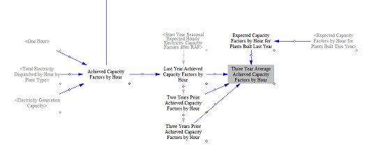
These values are also used to calculate average annual achieved capacity factors. We use achieved capacity factors because they can reflect the evolving nature of the power system and the impact to plant run times. For example, in a power sector decarbonization scenario, the achieved capacity factors for fossil thermal plants will decrease significantly. If we used a static capacity factor, then when computing anticipated revenue and costs for new power plant types, we would fail to capture the fewer hours those plants run. With achieved capacity factors, the model correctly tracks the evolution of the power sector composition and the impact this has on cost recovery for new power plant types. To calculate achieved capacity factors for new plants, we discount the expected capacity factor by the proportion of the three-year average achieved capacity factor to expected. For example, if natural gas combined cycle plants have a three-year average achieved capacity factor of 25% but their expected capacity factor is 50%, we reduce the achieved capacity factor for new plants by 50% (25% divided by 50%) to 25%.
These rely on weighted average data across the whole fleet by power plant type. In the start year we also compute start year capacity factors based on input data, since there is no historical year data to start calculating from.
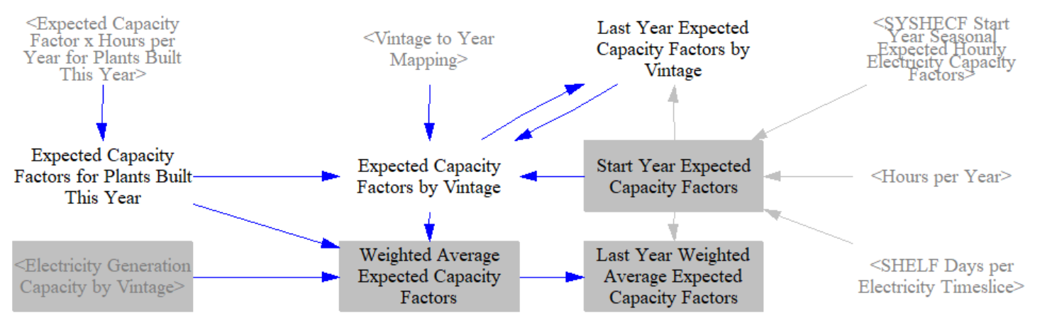
We also use expected capacity factors where there is no existing capacity from which to calculate an achieved capacity factor, for example novel technologies like hydrogen combustion turbines or small modular reactors. In these cases we compute a hypothetical capacity factor as if one megawatt of that power plant type had been available for dispatch.
Bid capacity factors are used in the dispatch mechanisms to reflect the available capacity in a given hour available to dispatch. They incorporate several limitations, including a maximum capacity factor, i.e. the maximum share of potential output that is available in each hour. Because the EPS is also a single-region model, we also include the ability to discount the available output to account for the regionality of the grid. If we didn't include this, the model would operate as a copper sheet with a power plant in one region being able to supply power in a wholly different region. These parameters are set through RAF Regional Availability Factor for Generation and are generally handled through calibration. Non-dispatchable renewables are not typically affected by this calibration. Capacity factors used for reliability calculations (i.e. that reflect an equivalent to effective load carrying capacity) are calculated here as well. This effective-load-carrying-capacity adjustment is applied separately to generation sources and to demand-altering technologies (such as demand response, EV batteries, and storage), reflecting the different ways each contributes to meeting peak reliability needs.
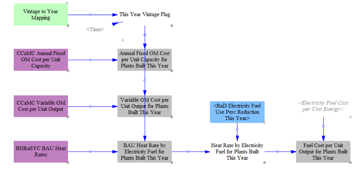
Other Weighted Average Fleet Properties
We compute values for new plants, including fixed O&M, variable O&M, and heat rates. We use this to also compute the fuel cost for newly built power plants.
The model next moves to computing properties for the existing fleet on a weighted average basis to collapse plant vintage down into a single element for model runtime.
First we compute the weighted average heat rate for the fleet and generation costs per unit output.
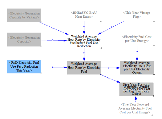
Next we compute the remaining properties for the existing fleet.
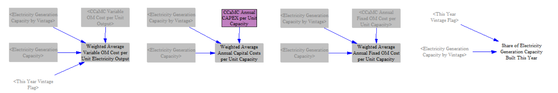
The model also calculates subsidies for electricity generation on a weighted average basis. We account for the duration of subsidies here as well, since some regions have subsidies that are limited in duration. We then have a weighted average across all the vintages for a single value by power plant type.
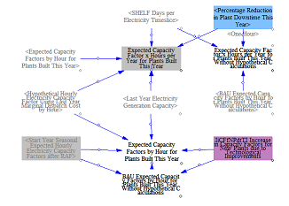
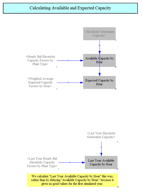
Available and Expected Capacity by Hour
Lastly, we compute the expected and available capacity by hour. Available capacity reflects the maximum available while expected reflects expected output, for example from hydro facilities where expected output is often far below maximum potential output.
Electricity Dispatch
At this point, the model has now estimated load, costs, retirements, capacity additions and retrofits and fleetwide properties, such as dispatch costs. The next step is to compute what is dispatched.
There are multiple dispatch mechanisms in the EPS, each with a specific purpose. The dispatch process begins with guaranteed dispatch, which is not price-based but rather is based on input data and policy drivers. This can be used to reflect, for example, equal shares dispatch. It can also be used for plant types that are typically price-insensitive, such as nuclear and on-site cogeneration facilities, such as biomass combined heat and power plants.
Following guaranteed dispatch is dispatch of RPS qualifying resources. This happens upstream of economic dispatch because there are instances where high-priced clean energy sources are needed to comply with the CES that may not dispatch if left solely to market dynamics.
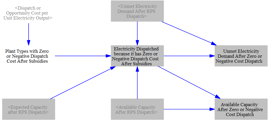
Next the model has a dispatch mechanism for negative- or zero-cost resources, i.e. those resources that have zero or lower dispatch costs. This step is needed due to mathematical limitations in the least cost dispatch step.
Finally, the model estimates least cost dispatch based on the marginal dispatch cost of resources.
The model does this using annual fuel price data to estimate actual dispatch and also using five-year average dispatch data to estimate a long run average dispatch amount for use in planning new resources.
The model combines all the dispatch data at the end of the dispatch process to compute a market price in each hour on an annual and five-year average basis.
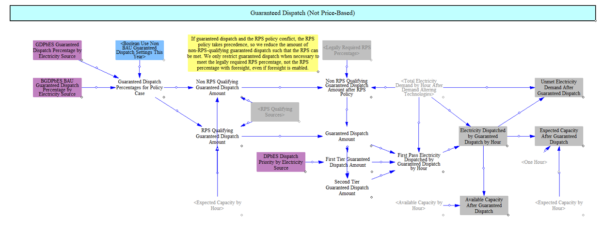
Guaranteed Dispatch
The model begins by dispatching resources that are guaranteed, as specified in input data. Based on this data, the model dispatches a fixed amount of the expected capacity of a resource in every hour. Expected capacity factors are based on input data and calculations described above for expected capacity factors. The input data can be configured to have two priority tiers so that in instances where the total amount of demand would be exceeded by guaranteed dispatch, it will first curtail resources in the lower tier and then the higher tier. In instances where guaranteed dispatch and the portfolio-standard mechanism (RPS or CES) conflict, the portfolio-standard mechanism will take precedence to ensure compliance.
Dispatch of Portfolio-Standard Qualifying Resources
Next the model will dispatch RPS- and CES-qualifying resources, starting with zero- and negative-cost resources and then moving to positive-cost resources. This step helps ensure that these resources are appropriately used even if their costs might exceed other resources. It also ensures alignment with the projected qualifying share as part of the CES/RPS optimization. The model uses available capacity factors for dispatch here. Because the expected and available capacity factors for variable renewables are the same, and most qualifying resources today are variable, this is generally not an important distinction, but it matters for certain resources like clean firm resources, which can be used at higher capacity factors when needed to meet CES/RPS requirements. RPS-qualifying resources are dispatched first; remaining qualifying-but-not-yet-dispatched CES resources follow, since CES qualifying definitions are typically a superset of RPS.
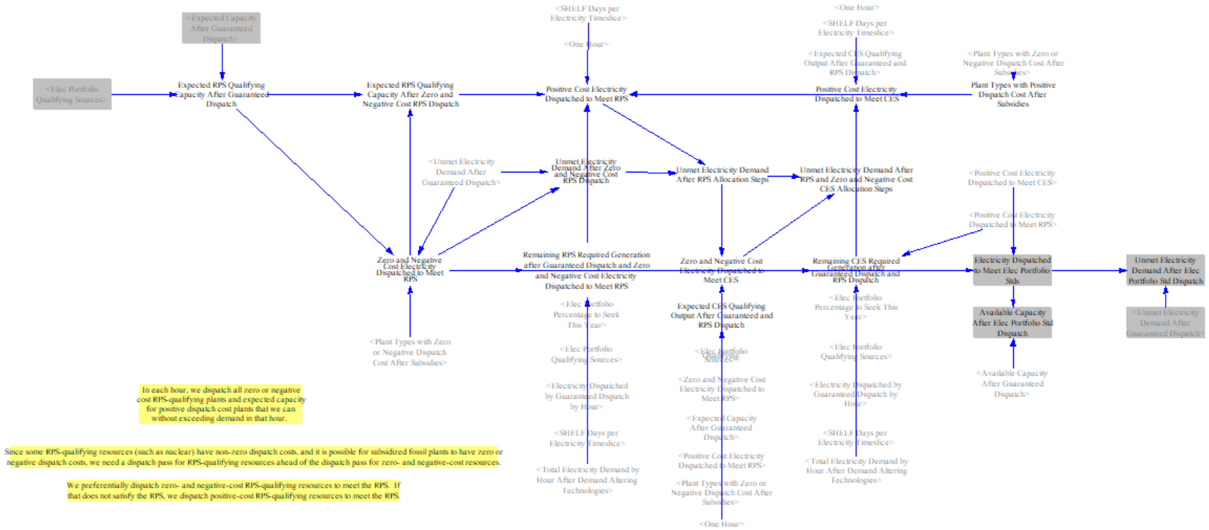
Dispatch of Remaining Zero- and Negative-Cost Resources
The model then moves to dispatching other zero- and negative-cost resources, since the least-cost dispatch mechanism is not able to accommodate resources with negative or zero marginal costs. They are dispatched at expected capacity factors. In instances where dispatching these resources would exceed demand, they are proportionally reduced so that supply and demand are in balance.
Least Cost Dispatch
Finally, the model calculates remaining dispatch through the least cost dispatch mechanism. This structure iteratively converges on an electricity market price that dispatches the right amount of electricity to meet remaining demand.
To do this, we start by representing each power plant type as a Weibull distribution. In reviewing real world data, we observed that dispatch costs most commonly represent different forms of Weibull distributions. We calculate the relevant parameters for each power plant type in the input data and use this, along with the dispatch cost per unit output (itself one of the parameters for a Weibull distribution) to compute a distribution for each resource. The model uses this information to estimate the share of each resource type that is dispatched at a given price and multiplies this by the remaining available capacity to estimate the output in any given hour for a given price. The mechanism runs through 20 optimization passes to converge on a market price where supply meets demand. This section also accounts for resources dispatched elsewhere so that the marginal dispatch cost reflects the marginal amount of supply available by resource type.
We limit the least cost dispatch mechanism only to resources identified in the input data as participating in least cost dispatch to significantly reduce the computational requirements, which are otherwise very high. Care is required to ensure that resources not flagged as participating in least cost dispatch are correctly dispatched elsewhere.
We also separately account for hydro dispatch as part of this mechanism by adding a “hydro opportunity cost” and allowing it to economically dispatch. This is required because while hydro plants have no fuel costs, they do have real opportunity costs they have to balance in determining whether or not to increase their dispatch and they are also a core part of flexible supply in certain geographies.
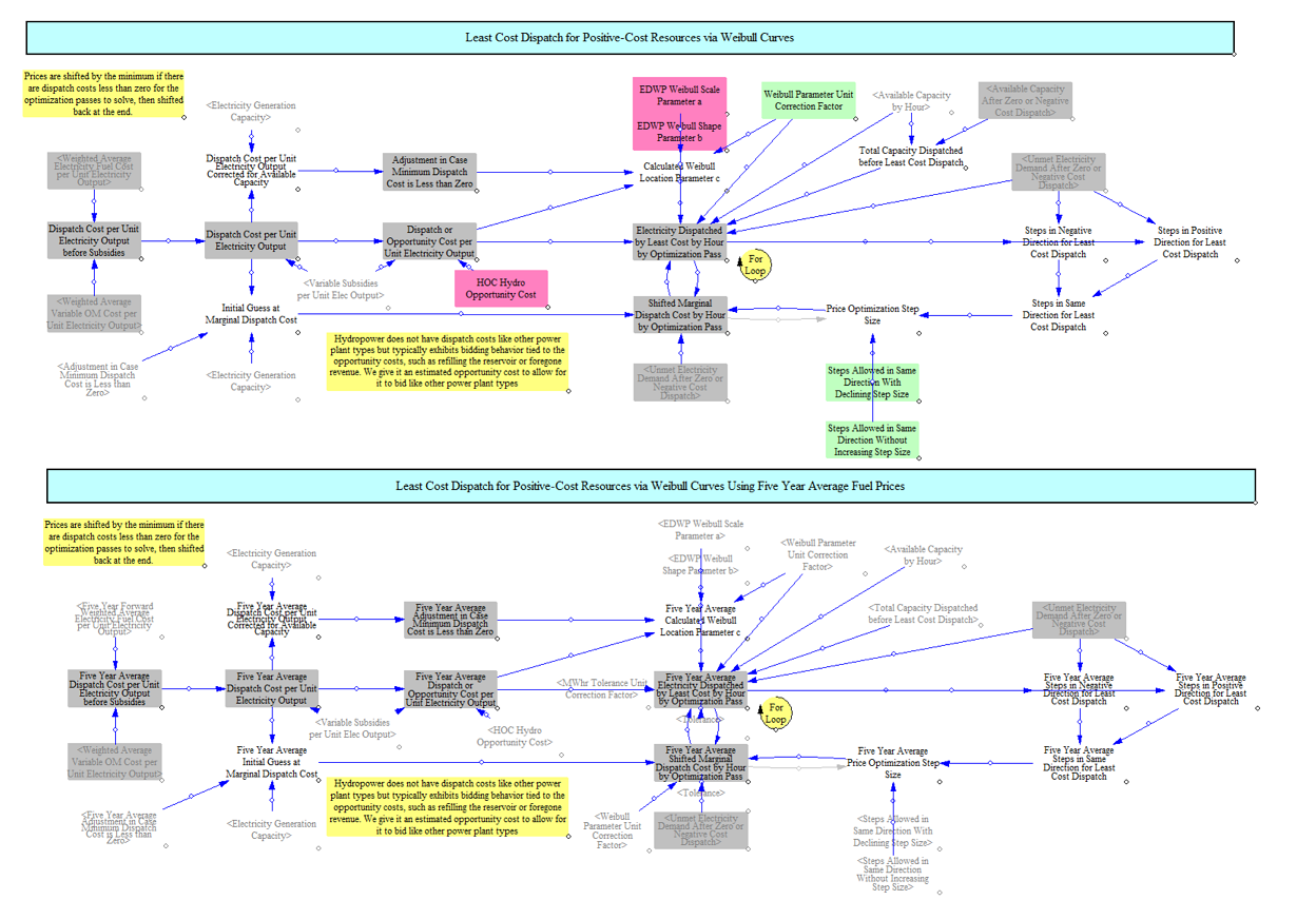
As mentioned earlier, we do least cost dispatches twice: once using annual dispatch costs and once using five-year average dispatch costs. The latter approach and accompanying market prices are used elsewhere in the power sector for determining future market revenues for new power plants. This avoids having a single year with high market prices used to represent anticipated future revenues.
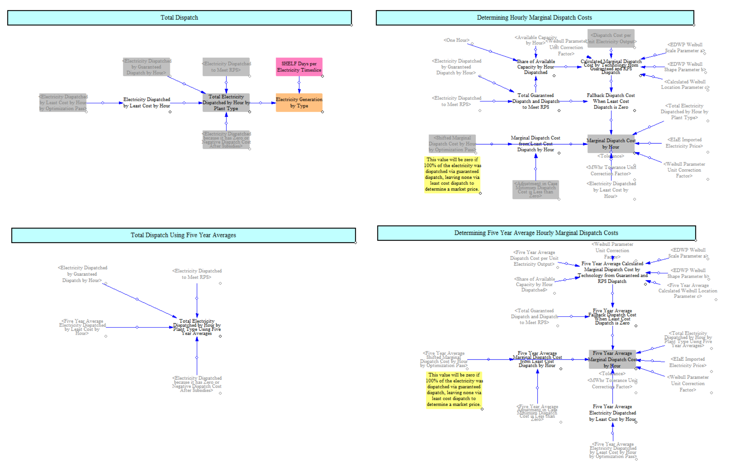
Summing Total Dispatch and Estimating Market Prices
Total electricity dispatched is summed across each of the elements of the dispatch pass. Dispatch estimates are used to compute market prices for every hour on an annual and five-year basis. In hours when there is electricity dispatched through least cost dispatch, the model has a calculated price from the least cost dispatch mechanism to use and will use the output of the least dispatch mechanism. However, there can be other hours in which there is no least cost dispatch, especially as the grid approaches 100% clean and most or all dispatch happens through the other dispatch mechanisms. In these hours, the model calculates a weighted average marginal dispatch cost of other resources to determine an “average” market price. Separately, particularly in small geographies, there can be hours in which all of the in-region supply is provided by imports. In these hours, we use the imported electricity price specified in input data.
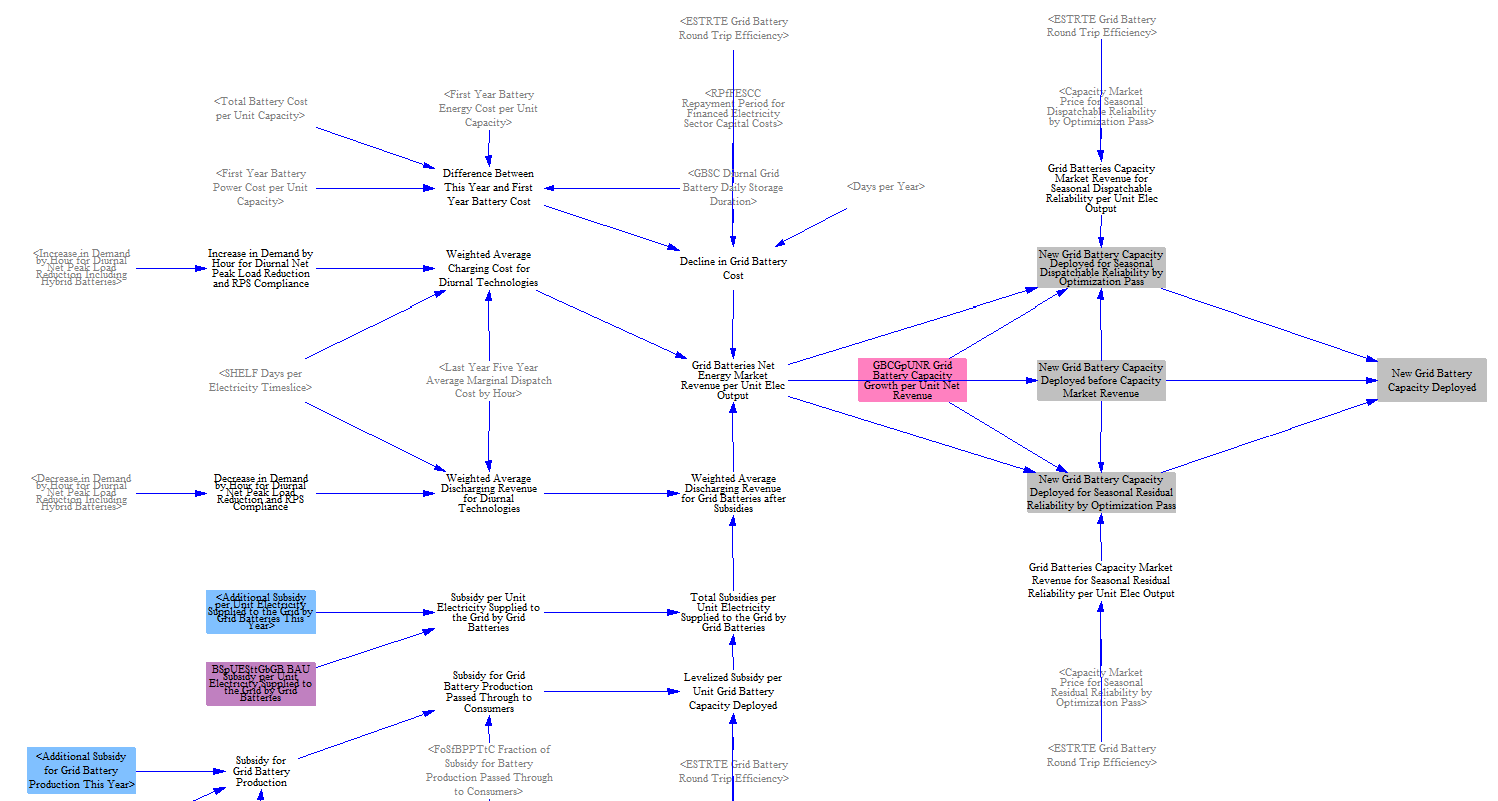
Economic Storage Additions
The electricity sector estimates economic additions of grid battery storage -- specifically standalone grid batteries (storage that is not co-located with a renewable power plant). Storage additions for hybrid power plants (renewables paired with on-site batteries) are co-optimized with the hybrid plant's capacity expansion in the cost-effectiveness step described above. The standalone grid-battery additions described in this section are tracked separately from hybrid storage and use a different revenue-driven methodology. Both standalone and hybrid storage are summed at the end for use in load shifting, market price formation, and reliability checks.
To estimate standalone grid-battery additions the model starts by calculating anticipated market revenues. Unlike for power plants, the model does not directly compare anticipated revenues and against costs to estimate additions, but rather looks only at the anticipated net revenue. This approach is necessary because the EPS omits several sources of revenue for storage, notably including ancillary services like frequency response, and comparing against costs would yield far lower profitability than in reality. Additionally, while the EPS now has hourly granularity for six electricity timeslices, to fully capture the revenue potential for storage would required sub-hourly detail, in addition to grid services. If we directly compared costs and revenues, we would miss a large source of revenue and significantly underestimate anticipated storage additions.
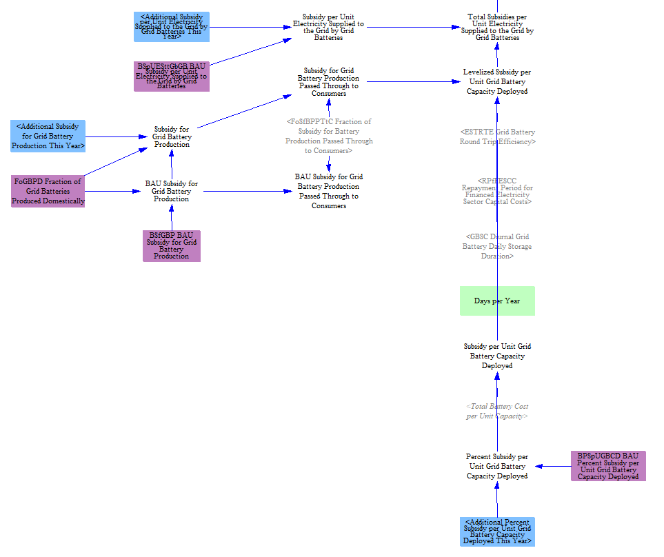
To estimate market revenues, the model compares the highest and lowest priced hours and computes an estimated daily profit by arbitraging these hours based on the duration of the storage (four hours by default in the US model). This allows the model to determine an estimated annual average charging and discharging profit per MWh of battery capacity. Incentive policies add to the profitability and drive additional storage capacity. Revenues from the reliability mechanism are integrated as well in this step. Declines in battery costs are modeled as a form of revenue as well to reflect increasing profitability of batteries. Together these elements comprise a "net revenue" estimate. The calculation of incentive policies, which can take the form of subsidies for production, for capacity installed, or per unit output, is shown below.
The total net revenue is multiplied by a calibrated input parameter (the MWh of storage added per $/MWh profit) to estimate battery additions. The storage additions are added to the model’s capacity on a one-year delay. Storage additions for the US and state models approximate those observed from other dedicated power system models, e.g. the National Renewable Energy Lab's ReEDS model.
Total Emissions
Next, we determine the pollutant emissions based on the generation by type, as shown in the following screenshot:
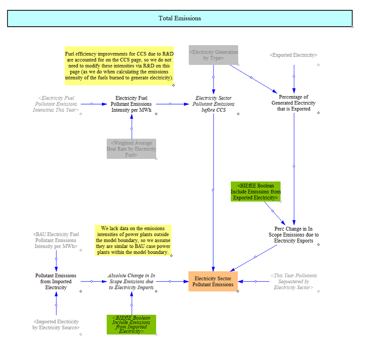
We use emissions indices (per unit energy in the fuel) and heat rates (energy units of fuel per MWh of electricity) to obtain pollutant emissions indices per MWh of electricity. We also apply any carbon capture and sequestration that is performed by the electricity sector, reducing CO2 emissions but also increasing fuel consumption (to power the CCS process). We apply the emissions indices per MWh to the total generation and add in the CCS effects to obtain an emissions total for the electricity sector by pollutant. The EPS also includes the ability to include or exclude emissions from either imported electricity or from exported electricity. These are control levers that are set separately through input data.
Additional Electricity Outputs
This section includes a few calculated variables that may be of interest in evaluating the electricity sector's performance or characteristics. Some of these values can be useful for debugging or evaluating the realism of the model's response to a given set of input data or policy settings.
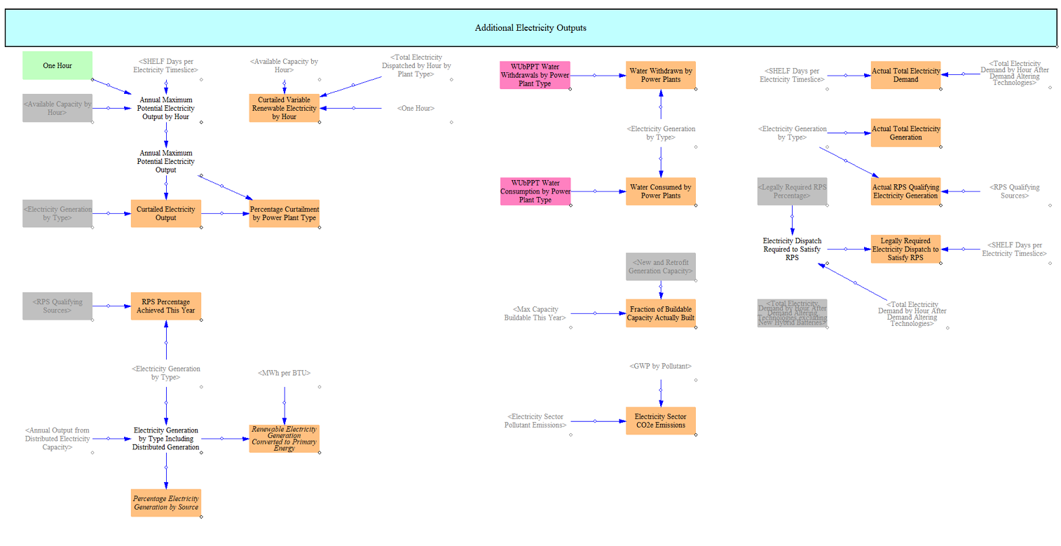
We calculate the amount of curtailed electricity output (based on the reduction in expected capacity factors) from each variable electricity source. These calculations are based on the expected output at expected capacity factors for these resources compared to their actual output. Curtailment can happen when supply is greater than demand or when other resources are guaranteed ahead of variable renewable resources.
We also track compliance with the RPS and CES, which are used by their respective optimization passes and the accompanying graphs. Conversions to other outputs, such as the percentage generation from clean sources and renewable electricity generation in primary energy units, are also handled here.
The EPS also tracks water withdrawn and used by power plants based on input data on power plant types and generation by power plant types.
Finally, the model aggregates pollutant emissions into estimate of CO2e and computes a few additional metrics used throughout the electricity sector.
This page was last updated in version 4.0.5.