Industry & Agriculture Sector (main)
General Notes
Included Industries
In the Energy Policy Simulator (EPS), the Industry Sector tracks emissions from the following specific industries or industry categories:
| Industry category | ISIC code(s) | U.S. model NAICS mapping |
|---|---|---|
| agriculture and forestry | 01-03 | 111–113, 1151–1153 |
| coal mining | 05 | 2121 |
| oil and gas extraction | 06 | 211 |
| other mining and quarrying | 07-08 | 2122, 2123 |
| food, beverage, and tobacco | 10-12 | 311, 312 |
| textiles, apparel, and leather | 13-15 | 313, 314, 315, 316 |
| wood products | 16 | 321 |
| pulp, paper, and printing | 17-18 | 322, 323 |
| refined petroleum and coke | 19 | 324 (refining, 32411, modeled separately in AEO's LFMM) |
| chemicals | 20 | 325 |
| rubber and plastic products | 22 | 326 |
| glass and glass products | 231 | 3272 |
| cement and other nonmetallic minerals | 239 | 327 except glass (e.g. 3271, 3273, 3274, 3279) |
| iron and steel | 241 | 3311, 3312, ferrous foundries 331510 (and merchant coke ovens, 324199) |
| other metals | 242 | 3313, 3314, nonferrous foundries 331520 |
| metal products except machinery and vehicles | 25 | 332 |
| computers and electronics | 26 | 334 |
| appliances and electrical equipment | 27 | 335 |
| other machinery | 28 | 333 |
| road vehicles | 29 | part of 336 (e.g. 3361–3363) |
| nonroad vehicles | 30 | part of 336 (e.g. 3364–3366, 3369; includes motorbikes) |
| other manufacturing | 31-33 | 337, 339, and asphalt (324121, 324122, 324191) |
| energy pipelines and gas processing | 352-353 | natural-gas processing and pipeline transport (≈ 2212, 486210) |
| water and waste | 36-39 | 2213, 562 |
| construction | 41-43 | 23 |
The ISIC codes are the EPS Industry Category subscript identifiers used throughout the model. The NAICS codes show the approximate North American Industry Classification System correspondence for the U.S. EPS: the industry breakdown largely follows the AEO Industrial Demand Module (IDM) categories (IDM Table 1), with a few categories combined or split to align AEO energy data with the U.S. Bureau of Economic Analysis (BEA) and Bureau of Labor Statistics (BLS) economic data the EPS uses. In particular:
- food, beverage, and tobacco, textiles, apparel, and leather, and the printing portion of pulp/paper/printing are separated out of AEO's "Miscellaneous finished goods" category (NAICS 312–316, 323) and reallocated by economic output.
- iron and steel versus other metals splits AEO's iron-and-steel, aluminum, and "other primary metals" categories — including ferrous (331510) versus nonferrous (331520) foundries — by output shares.
- road vehicles versus nonroad vehicles splits AEO's transportation-equipment manufacturing (NAICS 336) by output shares; "nonroad vehicles" here includes motorbikes.
- other manufacturing is the residual of AEO's "Miscellaneous finished goods" (furniture, NAICS 337; miscellaneous, 339; asphalt, 324121/324122/324191) after the reallocations above.
- oil and gas extraction additionally absorbs natural-gas lease and plant fuel, while energy pipelines and gas processing and water and waste are not standalone AEO IDM manufacturing industries and are derived from other sources, so their NAICS correspondence is approximate.
Note that 'agriculture and forestry' is treated as a specific industry. Though this industry category does include the economic activity related to forestry, it is distinct from the emissions and cash flow calculations in the Land Use, Land Use Change, and Forestry (LULUCF), which is handled on its own LULUCF Sector page.
Not every industry category listed above will be used in every region depending on data availability. Where data for not all 25 industries is available, data for multiple categories may be grouped together (for example, some regions may group 'road vehicles' and 'nonroad vehicles' together into a single 'vehicles' category).
Types of Emissions
Two types of emissions are tracked in the Industry Sector: energy-related emissions and process emissions. Energy-related emissions are similar to emissions from other sectors in the model; they come from the combustion of fuel to generate energy that is used to provide specific services (in this case, to manufacture industrial products). It does not matter if the fuel is combusted to create usable heat, on-site electricity, or some other form of energy: this is considered fuel use by industry. This means that the electricity use by industry shown in the EPS refers to electricity obtained from the grid, not electricity generated on-site using fuels, waste heat, or other means.
Process emissions refer to the emissions of any of the twelve tracked pollutants that occur as a result of industry operations and which were not related to the combustion of fuel for energy. For example, when limestone is chemically broken down as part of the cement-manufacturing process, the CO2 that is released is an example of process emissions. Similarly, when methane leaks from wells or pipes, the leaked methane is process emissions. Sometimes a high-GWP gas is itself an industrial product, such as various hydrofluorocarbons (HFCs) that are used as solvents, fire suppressants, refrigerants, and propellants; these also count as process emissions.
Foreign Leakage
The EPS considers policies only on a regional scale. Typically, a unilateral policy that lowers emissions from industry will lead to an increase in emissions in other nations. This can happen because some companies move their operations overseas, or because companies that are already overseas scale up production (to export to the modeled country -- in this case, to the U.S.) and domestic manufacturers reduce production.
In certain cases, leakage can be negative. That is, a reduction in emissions from the modeled country also leads to a reduction of emissions from other countries. This is most likely to happen if the modeled country (the U.S., in this case) is a major player in setting the market price for a globally traded commodity. When policies within the U.S. cause the U.S. to reduce production, the global price for the good increases due to the reduction in supply. As a result of the higher prices, consumers in other countries reduce demand for the product. In the case of the U.S., production of coal, oil, and gas all have negative leakage rates, whereas nearly all other products have positive leakage rates.
Emissions due to leakage are estimated by the model but are not added to total emissions, since that total is meant to reflect only emissions from the modeled country.
Changes in Industrial Production Levels
Changes in Imports and Production for Nonfuel Industries
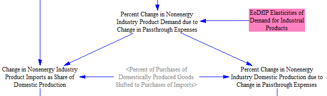
The EPS reads in input data on industrial production, imports, and exports to help construct its BAU case. However, it is important to track any policy-induced changes to these amounts, particularly for domestic production (which causes changes in domestic fuel consumption and industrial emissions). The model allows policies to influence the level of industrial production via several mechanisms. The first mechanism works by changing nonenergy industrial production in response to changes in industry expenses due to policy. When an industry's expenses increase or decrease, it will often "pass through" those expenses to buyers, either increasing or decreasing the cost of industrial goods to reflect the new cost to produce those goods. Policy-induced changes in industrial expenses in the EPS are due to changes in spending on fuels (through policies like industrial efficiency that lead to reduced fuel consumption or policies that adjust fuel prices like a carbon or fuel tax), carbon taxes on process emissions, capital expenses due to efficiency or fuel shifting policies, implementation costs of process emissions policies, carbon capture equipment and O&M costs, and any carbon tax rebate from carbon capture. To find the percent change in costs for each ISIC code, we divide by industrial output, which is calculated in the Input-Output Model (we implement a one year delay in output to avoid circularity). Because our input data on industrial output does not include value-added tax (VAT) or sales tax, we remove any VAT or sales tax from the expenses passed through to buyers before dividing by output.
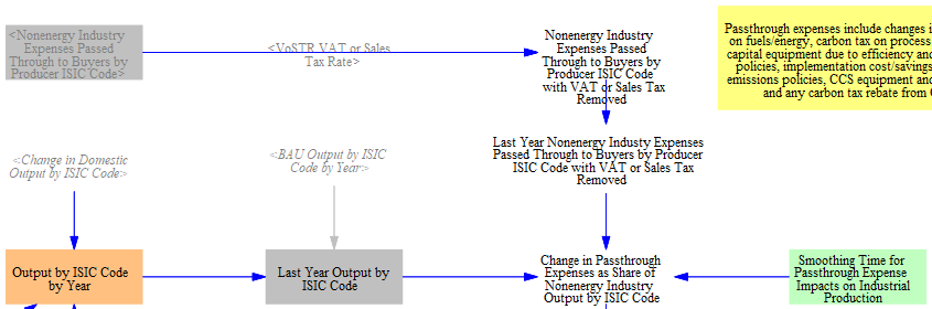
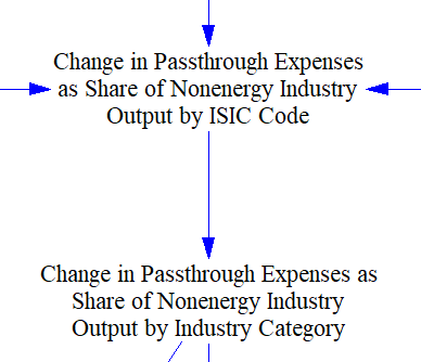
We then map the changes in expenses for each ISIC code onto the relevant industry category. In general, the industry categories tracked in the EPS align directly with one of the tracked ISIC codes. However, the full list of ISIC codes is broader than the tracked industries, since ISIC codes include services such as education and human health and social work.
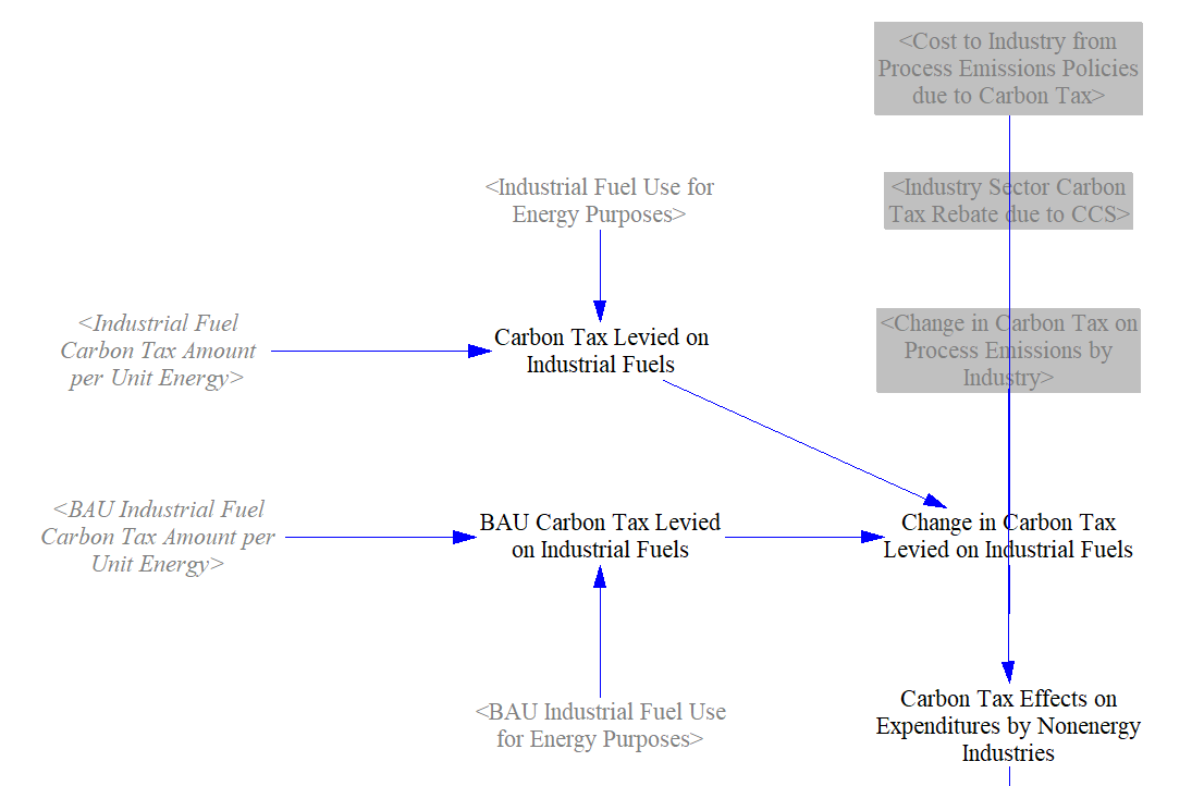
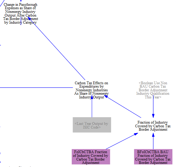
The EPS allows for a Carbon Tax Border Adjustment, which applies fees on imported goods based on their carbon content. If the Carbon Tax Border Adjustment is enabled, then we remove any carbon tax effects on industry expenditures from the change in passthrough expenses calculated above. This is because when calculating changes in industrial production, we want domestically produced goods competing equally with imported goods, and we don't have the necessary input data to calculate the carbon content of all imported goods (which may come from many different countries with different carbon intensities of production). We therefore need to calculate the carbon tax effects on industry expenditures. To do this, we first sum the change in carbon tax levied on fuels, change in carbon tax on process emissions (if the carbon tax applies to these emissions), the costs to industry from implementing process emissions measures due to a carbon tax, and any carbon tax rebate due to carbon capture and sequestration.
We then multiply the calculated carbon tax effects by the "Share of Change in Industry Expenses Passed Through to Buyers," which is read in as input data. By default, we set this value to 1 to represent full passthrough of changes in expenses to buyers based on the literature.

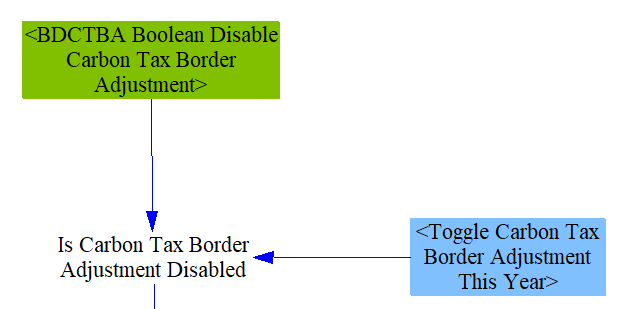
We can now remove the calculated carbon tax effects from the industry's change in passthrough expenses, if relevant. We check to see whether the Carbon Tax Border Adjustment is disabled in each year. Whether or not the Carbon Tax Border Adjustment is enabled by default is set through the control setting "BDCTBA Boolean Disable Carbon Tax Border Adjustment," and users can then decide whether to toggle the adjustment on or off through a policy lever. This behavior can be customized through implementation schedules, meaning a user could institute a Carbon Tax Border Adjustment partway through the model run.
If the Carbon Tax Border Adjustment is enabled in a given year, the calculated carbon tax effects are removed from change in passthrough expenses as a share of output. Two input files allow the user to define the share of each industrial sector's output that are covered by CBAM and to change these values in the policy scenario through a boolean lever. This might help a user reflect the EU's CBAM better, for example, as only fuels used for production of certain chemicals are covered by the CBAM. In effect, then, only a share of the carbon tax's effects on that industry would be removed from passthrough expenses.
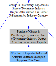
Next, we calculate the effects of the Buy In-Region Products policy. This policy shifts the specified fraction of imported industrial output to in-region suppliers. Before we calculate the effect of import substitution due to changes in price, we need to remove the fraction of imports shifted in-region.
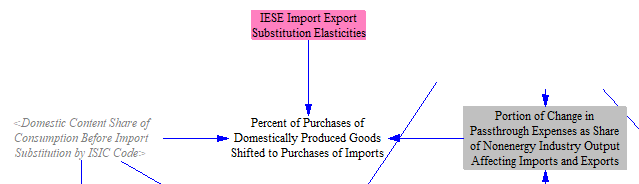
We now apply 'IESE Import Export Substitution Elasticities,' also known as Armington elasticities. These elasticities are set for each nonenergy industry and represent the elaticity of substitution between goods produced in different countries, meaning we calculate the percent of domestically produced goods shifted to imports in response to higher or lower prices. When applying the elasticities to the calculated portion of passthrough expenses affecting imports and exports, we make sure the domestic content share of production is between 0 and 100 percent. We will use this calculated 'Percent of Purchases of Domestically Produced Goods Shifted to Purchases of Imports' below when calculating the total change in imports and production.
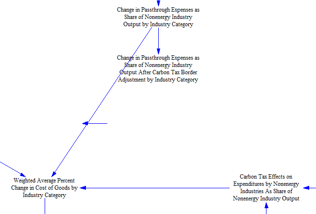
For our next step, we first need to calculate the 'Weighted Average Percent Change in Cost of Goods by Industry Category,' accounting for the change in passthrough expenses for domestically produced goods and the carbon tax effects (if applicable) for imported goods.
We can now calculate the change in overall product demand, which will flow through to both the demand for domestically produced and imported goods. Here, we use a separate set of elasticities that reflect the change in demand for industrial products in response to price (rather than the elasticity that reflects import substitution for domestic products to meet demand).

We then use this calculated change in demand along with the percent of domestically produced purchases shifted to imports to find the change in imports and the change in production. We assume that reductions in demand affect domestic production and imports equally (meaning each is reduced by the same percentage).
We now have the information we need to calculate the total imports of nonenergy products. We calculated the change in imports as a share of domestic production above, so we can multiply by domestic output to find the total change in imports in dollar terms. We can also add that to BAU imports to find 'Imports of Nonenergy Products.'

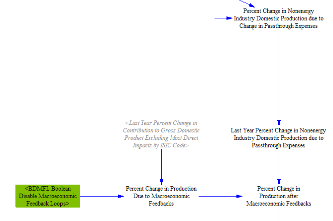
However, there are a few more required steps before finalizing the total change in domestic production. First, we adjust production for macroeconomic effects from the Input-Output Model (see the Macroeconomic Feedbacks page for a detailed discussion). This step implements a one-year time delay to avoid circularity when adjusting demand for nonenergy products by indirect and induced economic contribution to Gross Domestic Product. The 'Boolean Disable Macroeconomic Feedback Loops' control setting shown below can be used for debugging purposes, but most users will not need to disable this feature and will want to inlcude its effects.
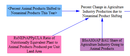
We then apply two policies that affect demand for nonenergy industrial products. The first is the Shift to Non-Animal Products policy, which works by setting a percentage shift away from animal products and toward plant-based replacements. This involves both a reduction in animal agriculture and an increase in other agricultural goods to replace that lost nutrition. To account for this, we use input data on the share of the agriculture industry made up of animal products and the 'Ratio of Nutritionally Equivalent Plant to Animal Products Produced per Unit Land Area.' This input data will vary by region, as it uses historical data on the types of animal products produced and a study that reports the opportunity food loss from production to final consumption for the five major animal product categories and their plant-based replacement diets.
The final adjustment is for the Material Efficiency, Longevity, and Re-Use policy, which buckets several approaches such as producing the same products using less material, reusing materials, and reducing the need for new industrial products. It is likely most relevant for industries like cement and iron and steel, which provide the raw materials for a large portion of construction and have significant potential for material efficiency. Users set the desired percentage reduction in production by industry category, which is directly applied on top of the changes in production calculated above.

The final variable 'Percent Change in Nonfuel Production due to Policies' will be used later in the Industry and Agriculture - Main sheet to adjust industrial energy use and emissions in response to policy.
Changes in Exports and Domestic Consumption for Nonfuel Industries
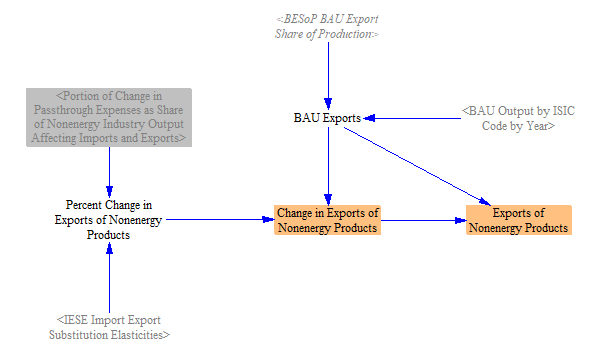
The Armington elasticities we use in the input data variable 'Import Export Substitution Elasticities' can be used to calculate both changes in imports and exports, since a change in the price of exported goods will affect demand for those goods abroad. As we did for imports, we can also multiply the change in industry passthrough expenses by the Armington elasticities to find the 'Percent Change in Exports of Nonenergy Products.' We have input data on the amount of BAU exports by industry category, which allows us to also calculate the change in exports in dollar terms as well as the total amount of exports.
Finally, we know that domestic consumption of goods will always equal domestic production + imports - exports. We have already calculated changes in production, imports, and exports, meaning we have enough information to calculate both Domestic Consumption of Nonenergy Products and the Change in Domestic Consumption of Nonenergy Products. Note that the variables for production shown in the screenshot below are sourced from the Input-Output Model sheet, where a full accounting of changes in output by ISIC code occurs.

Change in Production for Fuel Industries
The Fuels page includes a detailed accounting of production, imports, and exports of each fuel type tracked by the model. We want to add the calculated change in domestic fuel production to our calculated changes in nonenergy production so that we have a variable that tracks all 25 industry categories, which we label 'Percent Change in Production due to Policies.' The screenshot below shows the relevant structure. Note that the 'Percent Change in Domestic Fuel Production by Fuel' variable contains the change in electricity production even though it is not used in the Industry and Agriculture - Main sheet. This is because it is used in the Industry and Agriculture - Cash Flow sheet.

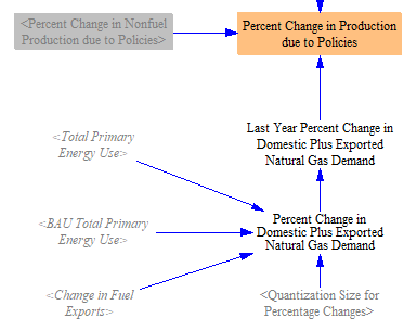
We then map the changes in production by fuel type to the relevant fuel producing industry categories, which are coal mining, oil and gas extraction, refined petroleum and coke, and energy pipelines and gas processing.

Because changes in production by fuel industries affect electricity demand and therefore which plant type are built in the Electricity Sector, they also affect domestic fuel use. We resolve this circularity with a one-year delay in this feedback, using 'Last Year Percent Change in Domestic Fuel Industry Production.' We add this to the 'Percent Change in Nonfuel Production due to Policies' to find 'Percent Change in Production due to Policies' for all 25 industry categories.

The one exception is for the "energy pipelines and gas processing industry," where we base changes in production on the change in demand for natural gas, not the change in production of natural gas. This is because there are EPS regions (such as U.S. states) which produce little or no gas, but can still have methane leaks from natural gas transmission systems. Using changes in natural gas demand better reflects changes in leakage from these transmission systems. As above, we institute a one-year time delay for this feedback.
Policies Affecting Fuel Use
Now that we understand any policy-induced changes in industrial production, we can begin to calculate industrial fuel use and emissions from that production. We calculate fuel use, allowing the user to enable a variety of policies that can affect the amount of industrial fuel consumption.
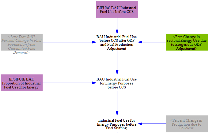
First, before we account for any policies, we want to establish the BAU fuel use. However, there are two types of industrial fuel use: fuel use for energy purposes and fuel use for non-energy purposes (or feedstocks). We track these two quantities separately so that we can correctly calculate emissions from fuels that are combusted for energy purposes later, as opposed to feedstocks which are not combusted (for example, petrochemicals that are incorporated into plastic products). We take in data on total industrial fuel use as well as the proportion of that fuel used for energy. The fuel used for non-energy purposes is temporarily removed in the screenshot below, and the portion used for energy purposes is multiplied by the percent change in production, the calculation of which is described above. This section also adjusts BAU fuel use for the 'Exogenous GDP Adjustment,' which is no longer used in the U.S. model. This feature can be used to adjust energy and service demand for the COVID-19 induced recession or other economic shocks that are not reflected in collected input data. Because the U.S. EPS input data already reflects COVID-19, we no longer rely on this feature. However, it is still in use in certain international EPS models.
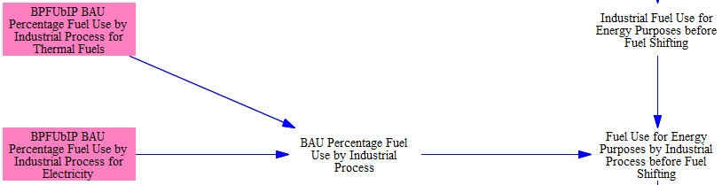
We can now adjust industrial fuel consumption using the first fuel shifting policy lever. The various fuel-consuming processes carried out in industry have heterogeneous demand for various fuels and differing potential for shifting to lower-carbon alternatives. For example, for low-temperature heat requirements, industrial heat pumps are the most efficient and cost-effective option. Higher temperature processes may require other electric heating technologies such as electric reistance or induction, or the combustion of a zero-emissions fuel such as green hydrogen. Other end-uses like electrochemical processes can only use electricity. Accordingly, we break out thermal fuel and electricity consumption by industrial process in each industry using input data. This allows us to apply fuel shifting policies to specific end-use processes.
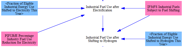
With industrial processes disaggregated, we turn to the implementation of fuel-shifting policies. Users can specify the amount of desired fuel shifting in each industry category and process. Fuel shifting will be applied to all fuels labeled as eligible in the input data variable 'Industrial Fuels Subject to Fuel Shifting.' As electrical processes are more efficient than those powered by combusting thermal fuels (heat pumps vs. boilers, for example), we apply a percentage industry fuel use reduction multiplier that reduces the input energy needed per unit output. This adjustment is subscripted by process.
Users can also specify that a portion of thermal fuel use be shifted to hydrogen combustion. The structure below shows how the EPS tracks both increases and decreases in each fuel type based on the user's policy settings, then calculates the total change in industrial fuel use from fuel shifting.
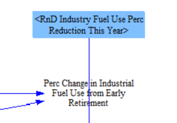
Subsequently, the model tracks the impact of various policies that lead to greater energy efficiency. The early retirement policy causes older, less efficient industrial facilities to retire before their normal lifetimes are exhausted. It does not affect production, which means that either new, efficient facilities are opened to replace them, or production levels are scaled up at existing facilities. The policy is implemented as a fraction of potential fuel use reduction achieved. The following screenshot shows the relevant structure:
The next policy represents measures taken to improve the design of industrial facilities as integrated systems, and to ensure all of the components of those systems work well together, and the flows between them are well-handled. This is distinct from any improvements to the components themselves (like motors, pumps, etc.), which is covered by the efficiency standards policy (discussed below). The policy is implemented as a fraction of potential fuel use reduction achieved. The following screenshot shows the relevant structure:
The next policy causes the adoption of more cogeneration and waste heat recovery than in the BAU case. Cogeneration refers to facilities creating both electricity and useful heat from the same process, while waste heat recovery refers to facilities making use of heat generated by various processes (such as the heat in an exhaust stream) to serve a useful purpose, such as to create electricity. In either case, it reduces the amount of fuel or grid-source electricity needed by industrial facilities. The policy is implemented as a fraction of potential fuel use reduction achieved. The following screenshot shows the relevant structure:
The industrial equipment efficiency standards policy specifies a required reduction in fuel use (relative to BAU) that will be mandated by standards for energy-using industrial components, such as motors, pumps, boilers, etc. This policy refers to the components that are assembled together as part of industrial facilities; efficiency improvements from improved installation practices or the proper integration and coordination of different components are handled by the installation and system integration policy (discussed above). Standards do not require facilities to retire early, mandate the use of cogeneration or waste heat recovery, or specify which fuel must be used, so the efficiency standards policy effects are non-overlapping with other industrial fuel use policies. The user specifies the percentage fuel use reduction required by the standards (subscripted by industry category and fuel type), so no input variable is necessary to convert a user setting into an energy usage value. The structure for the standards policy is shown in the following screenshot:
The R&D policy reduces fuel use by a user-specified percentage. As with other R&D policies, this policy represents additional R&D, beyond any that is required to comply with other policies, such as fuel efficiency standards. The following screenshot shows the relevant structure:
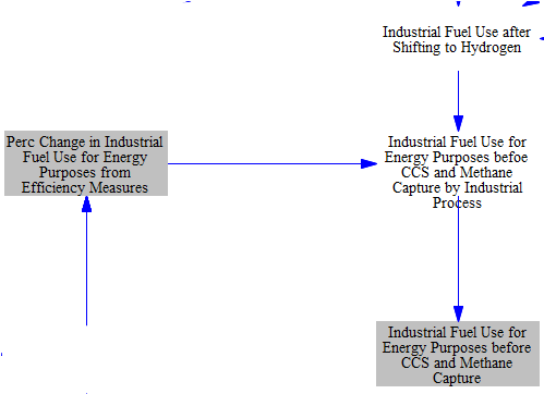
The impacts of each of these levers impacting efficiency are summed, accounting for the fact that multiple of these policies may be enabled at once. This gives us the percent change in fuel use due to energy efficiency measures. This percent change is multiplied by the fuel use calculated after fuel shifting, yielding total industrial fuel use for energy purposes, not including any fuel used for CCS or methane capture, both of which are handled later on.
Process Emissions
Policies
All but two policies affecting process emissions are represented as a fraction of the total potential abatement from that policy that is achieved (based on the user's policy setting and policy implementation schedule), so they are all handled via a similar calculation flow, as shown in the following screenshot:
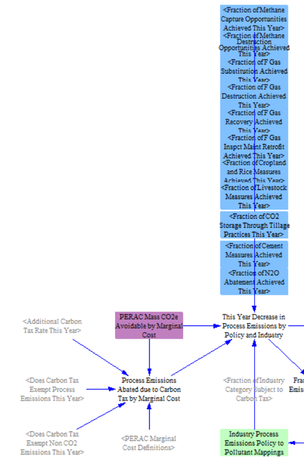
Each policy setting at its current year value is multiplied by the total potential reduction (in CO2e terms) in that year year to obtain reductions due to that policy (in CO2e). The total potential reduction is defined by the input file "PERAC Mass CO2e Avoidable by Marginal Cost", which projects the process emissions that can be abated by policy in the BAU.
Emissions reductions are disaggregated by industry and by policy. We include a helper variable 'Industry Process Emissions Policy to Pollutant Mappings' to assign the emissions abatement from each policy to the correct pollutant. Generally, each process emissions policy targets a single pollutant, for example substitution of f-gases in the chemicals industry or methane capture for natural gas and petroleum systems. The exceptions are the agricultural policies targeting cropland and rice and livestock, which include abatement of both CH4 and N2O. We apportion emissions reductions between these pollutants based on their share of BAU agricultural emissions.
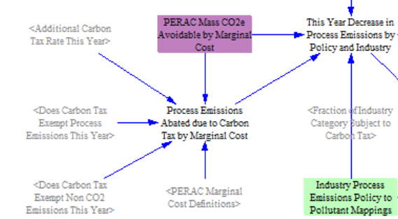
Our sources for potential percentage reductions achievable also break down the abatement potential into cost buckets, and the cheapest options are implemented first (see the Industry - Cash Flow sheet. If a carbon tax is enabled and applies to a source of emissions (which depends on whether the carbon tax is set to apply to process emissions and/or to non-CO2 gases), we also calculate the process emissions abated due to the tax. We assume that any abatement potential at a cost less than or equal to the carbon tax is implemented (including any potential that is negatively prices, or cost-saving). Emissions abated due to the carbon tax are then added to the variable 'This Year Change in Process Emissions by Policy and Industry.'
Next, we implement the Shift to Non-Animal Products policy. We multiply the user's setting for the percent of animal products shifted to non-animal products in each year by the share of agricultural process emissions from animals (specified via input data). Any emissions increases due to additional production of non-animal products is already covered in the Changes in Industrial Production Levels section above.

Calculation of Process Emissions
Now that we have calculated the change in process emissions from all relevant policies, we calculate the total change subscripted by industry category, process emissions policy, and pollutant. We ensure that reductions do not exceed BAU process emissions of a given pollutant for a given industry, which can happen if input data for BAU process emissions and abatement potential use different sources. The exception is the Improved Soil Measures policy, which can sequester CO2 in soils and therefore result in negative emissions. The relevant structure is shown below.
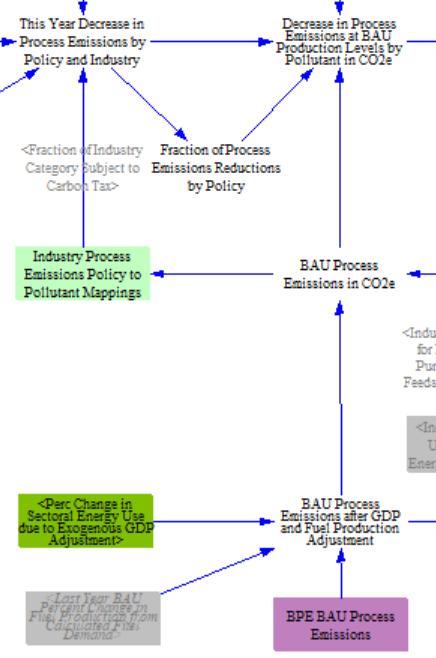
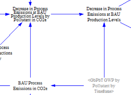
We then use global warming potential (GWP) factors to convert BAU Process Emissions in CO2e to BAU process emissions in units of each specific pollutant. (Here, we use the 100-year GWP timeframe, rather than the user-selected GWP timeframe, because the EPA source used 100-year GWP values when converting to CO2e, and we are simply undoing their conversion.)
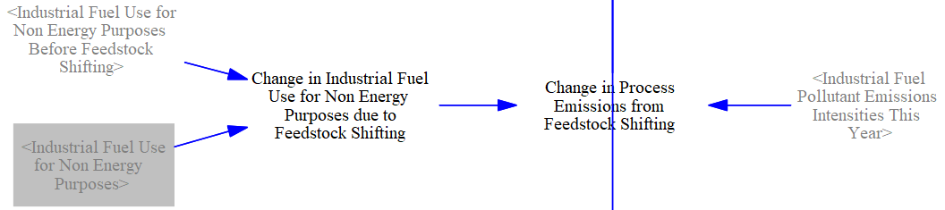
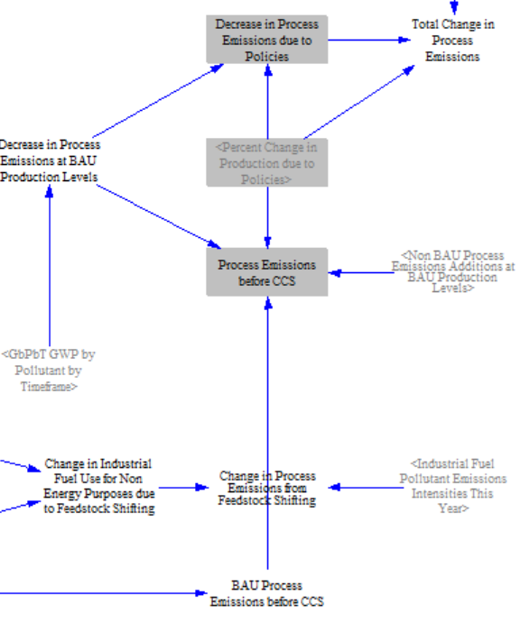
Next, we account for any changes in process emissions due to feedstock shifting. While all fuel-related policies to this point have tackled the impact of fuel use for energy purposes, we also include a policy -- described in the next section -- for reducing fossil feedstocks. This policy can represent the impact of a shift from oil and gas feedstocks in the chemicals sector (some carbon from which is are released as the feedstocks are chemically converted into other products) to hydrogen or biofuel feeds. It can also represent a shift from the use of metallurgical coal for iron reduction in primary steelmaking to direct iron reduction with hydrogen feedstock. In both cases, emissions arising during the production processes can be prevented by a change in feedstock. We use the change in fuel consumption for non-energy purposes and each fuel's representative CO2 emissions intensity to determine feedstock shifting's imapct on process emissions.
Then, we explicitly calculate non-BAU process emissions from input data, which can be enabled if a boolean policy lever is turned on by the user. This allows the user to explore differing projections of process emissions from various sources or the rollback of policies included in a BAU projection that would otherwise have lowered emissions and is subscripted by process emissions policy.
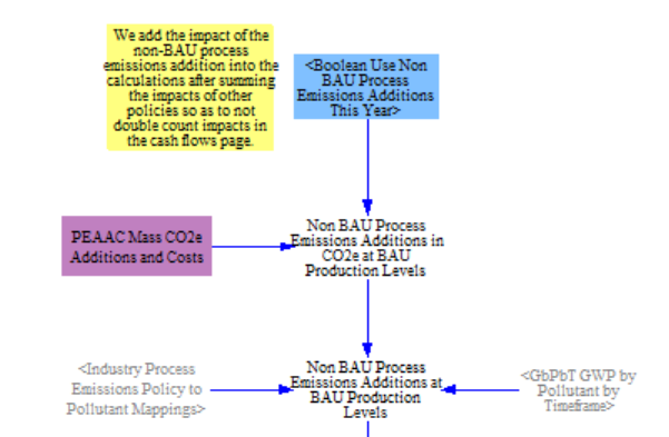
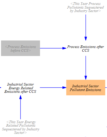
Finally, we apply the percent change in production due to policies (the calculation of which is explained above) to adjust both the process emissions and the change in process emissions to reflect increases or decreases in industry production levels. The 'Process Emissions before CCS' variable is used later on this sheet as a component of total Industry sector emissions, while the 'Change in Process Emissions due to Policies' variable is used on the Industry - Cash Flow sheet. We add in the non-BAU additions afterwards such that their cash flows can be calculated separately.
Totaling Fuel Use and Emissions
Fuel Use
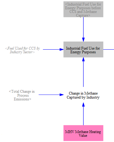
First, we find the total industrial fuel use for energy purposes. The calculations for most industrial fuel use are outlined above, but we need to add in two additional components. One is to add in the fuel used to power carbon capture and sequestration equipment in the industry sector, which is calculated separately on the Carbon Capture and Sequestration sheet. We also subtract out any methane captured through the Methane Capture policy (part of the process emissions calculations), since captured methane can be used to reduce that industry's non-feedstock natural gas usage (to a minimum of zero).
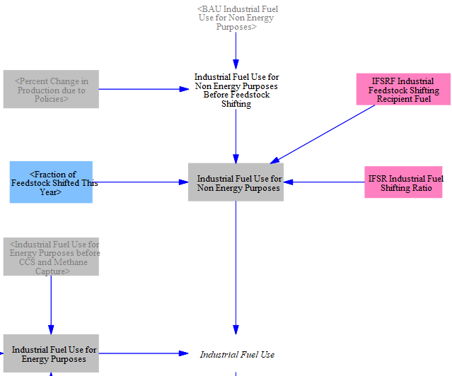
We then add back in the industrial fuel use for non-energy purposes (feedstocks), adjusting for the percent change in production due to policies and any shifting to alternative feedstocks, as defined by a policy lever and input data determining the recipient fuel and shifting ratio. This gives us our total 'Industrial Fuel Use.'
Electricity Demand
From the total industrial fuel use, we separate out the electricity demand and convert it to MWh. This refers to the electricity drawn from the grid (electricity that is generated and consumed on-site is not tracked as part of the "electricity" total because it does not require more power to be generated by the electricity sector). The following structure shows the reporting of electricity use:

Total Emissions from Industry (not including leakage)
Next, we convert fuel use for both industrial fuels used for energy purposes and fuels used to power industry CCS to emissions using the emissions intensities from the Fuels sheet.
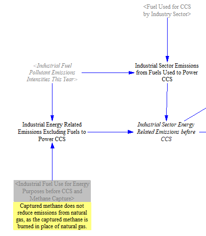
We then add process emissions and subtract the quantity of CO2 that is sequestered via CCS to give us total emissions from industry in the modeled region, as shown below. The structure separately subtracts CO2 sequestration from both energy related and process emissions before arriving at 'Industrial Sector Pollutant Emissions.'
Finally, we also create a variable that tracks industrial pollutant emissions in terms of CO2e for use in an output graph.

Foreign Leakage
The model calculates foreign leakage (emissions induced in foreign countries in response to unilateral implementation of policies in the model) via the following structure:
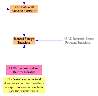
The difference between BAU and policy case emissions by industry are multiplied by the foreign leakage rate (by industry) to obtain the total induced foreign emissions. These emissions are not added into the totals for the modeled country or region- they are simply reported here. More information about the calculation of foreign leakage appears above on this page, under the "General Notes" header.
This page was last updated in version 4.0.4.