Buildings Sector (main)

General Notes

On this sheet, we calculate energy use and direct emissions from buildings and appliances. Rather than consider number of buildings, we break buildings down into six energy-using or energy-related components:

• heating
• cooling and ventilation
• envelope
• lighting
• appliances
• other energy-using components

Except for the "envelope" component, energy use is tracked on a BTU basis and is modified by various policies, such as efficiency standards, accelerated retrofitting, and component electrification. Envelope is used as a multiplier that affects the energy use of the "heating" and "cooling and ventilation" components. In the BAU case, this multiplier is 1. It can be improved via policies to represent improvement in the thermal insulation of buildings. After this process, the envelope number is multiplied by the "heating" and "cooling and ventilation" energy use figures to reduce their energy use if there were any envelope improvements. Thus, improvements for "heating" and "cooling and ventilation" components in this model refer specifically to the mechanical systems providing these services, and improvements resulting from improved insulation, windows, doors, etc. are handled via the envelope component. Users should keep this in mind when setting policy levers for each component type.

Note that water heaters, which are categorized as part of a building's "heating" systems in some data sources, are treated as part of the "appliances" component category in this model because water heater energy use should not be significantly affected by building envelope.

Estimating BAU New Components Energy Use

Our source data include projections for energy use, disaggregated by fuel type and by component. However, the source data do not specify what fraction of that energy use in each year is from new building components (i.e. those that entered service in the current model year, whether for use in new buildings or to replace old components in existing buildings). Most of the policies in the Buildings Sector affect newly sold components, so it is necessary to estimate the fraction of energy use each year that is due to these components. This estimate is handled via the following structure:

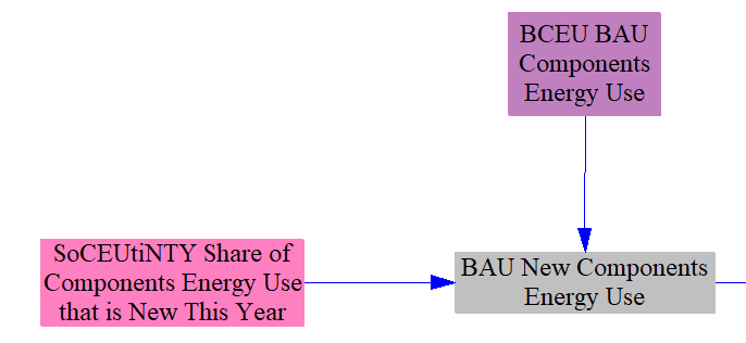
The input data variable 'Share of Components Energy Use that is New This Year' is based on the average lifetime of each component and adjusted during calibration to ensure there are no sharp discontinuities in energy use during the model run.

Policy Effects for New Components

Efficiency Standards and R&D

The following structure implements the energy efficiency standards and energy efficiency R&D policies for building components:

The implementation of these policies is straightforward, as the user settings of these policy levers explicitly define their effects. We conservatively assume that newly sold building components just meet the reduction in energy use required by the standard. The R&D policies are defined to be additional R&D beyond any that may be needed to satisfy requirements of other policies, such as R&D by building component manufacturers done in order to meet efficiency standards.

Improved Labeling and Contractor Education and Training

The following structure implements two Boolean policies (i.e., policies that can only be set to "on" or "off" rather than set to a range of different values): improved device labeling and improved contractor education and training.

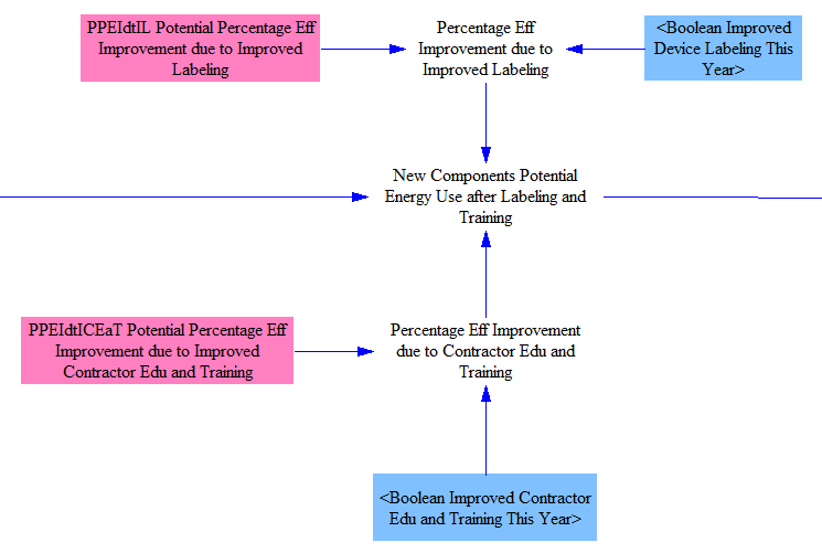
Energy efficiency labeling reduces the energy use of specific types of devices- appliances, heating equipment (i.e. central air furnace), and cooling / ventilation equipment (e.g. air conditioning units). Contractor education and training improves the performance of building envelope components, reducing energy spent on heating and cooling. In both cases, these are Boolean policies because specific labeling interventions and specific training programs were studied in our input data sources; it does not make sense to allow a user to implement a fraction of a labeling program or a fraction of a training program.

Rebate Policy and Component Quality Levels

The EPS supports multiple quality levels for building components. For the U.S. version of the simulator, there are only two quality levels: standard-compliant and rebate-qualifying. The structure that handles these quality levels, as well as the rebate policy, is shown in the following screenshot:

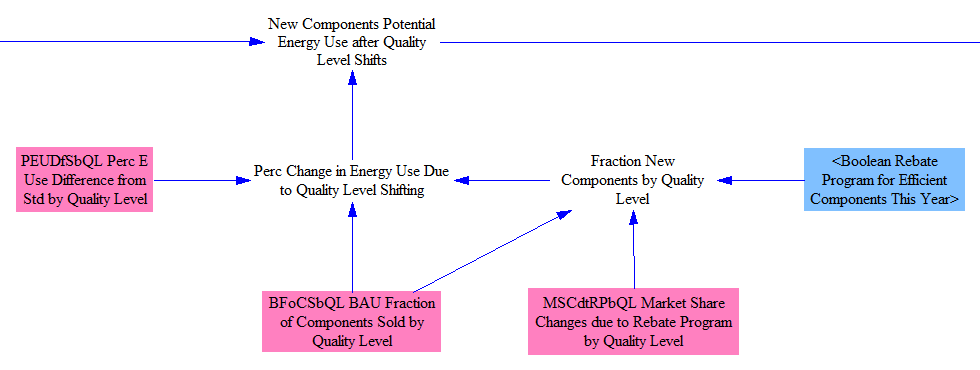
When the rebate policy is disabled, "Fraction New Components by Quality Level" and "BAU Fraction of Components Sold by Quality Level" are the same, so there is no "Perc Change in Energy Use Due to Quality Level Shifting." When the rebate policy is enabled, specific market share changes by quality level occur, causing more components of higher quality levels and fewer components of low quality levels to be sold each year. The differences in energy use (to provide the same building services) are taken in as input data and typically relate to how the quality levels were defined. In the U.S. dataset, we use standard-compliant components vs. Energy Star components to define our categories and set our energy use differences by quality level, due in part to the availability of data regarding Energy Star market shares and energy use.

The rebate program is a Boolean lever because only rebates of particular magnitudes have been studied in the literature. Typical rebate values represented by this lever are $50-100 for a clothes washer and $25-50 for a dishwasher or refrigerator.

Effect of Fuel Price on New Component Efficiency

In response to higher fuel prices, individuals sometimes choose to buy more efficient components and manufacturers may choose to offer more efficient components for sale. Conversely, if fuel becomes cheaper, components with lower efficiencies are more likely to be purchased. The following structure handles this effect:

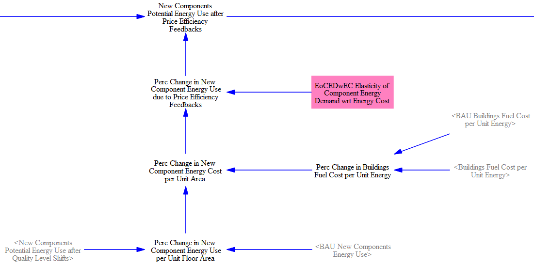
The energy use of new components is compared with the energy use of that same set of components after application of those policies that reduce the energy use of new components (such as efficiency standards, contractor training, etc.) to determine the "Perc Change in New Component Energy Use per Unit Floor Area." We don't actually work in terms of floor area -- this term is simply a way to express the fact that the components being compared provide services to the same set of buildings in the BAU and non-BAU cases, and we're capturing specifically the policy-caused energy efficiency improvements.

In the next step, we combine this change in energy use with the difference in fuel cost (disaggregated by fuel), which may be driven by other policies (such as a carbon tax or fuel taxes), most of which are handled on the Fuels page. This gives us a percentage change in cost to provide services to a given building area, disaggregated by component and by fuel type. We use an elasticity of new component energy demand with respect to energy cost to convert this into a percentage change in the energy efficiency of newly sold components. This percentage change is multiplied by the total energy use from the most recent prior calculation ("New Components Potential Energy Use after Quality Level Shifts") to give the potential energy use after price-efficiency feedbacks.

Fuel Shifting

A policy is available to shift newly sold components from their BAU fuel types to another fuel type, as shown below. This is typically used to represent electrification, but users can specify shifting to a different fuel source using the input data variable 'Recipient Buildings Fuel Fractions.'

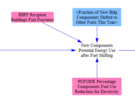
The implementation of this policy is relatively straightforward, because the user directly specifies the percentage of new components to be shifted to electricity (or other fuel source). The one complication is that we must make an adjustment to account for the fact that electricity is used more efficiently than other fuels on an energy unit basis (less heat losses, etc.). The fuel used to generate the electricity, and associated efficiencies, are handled in the Electricity Supply sector, not in the Buildings sector. (We make a very similar adjustment in the Transportation Sector and Industry Sector when implementing the other sector specific electrification policies.)

Envelope Effects

At this stage, we are done applying policies and economic effects that alter the efficiency and fuel use of new building components. The next step is to convert changes in envelope efficiency into changes in energy use, as envelope components do not themselves use energy. As noted above, envelope is handled as a multiplier that starts at '1' in the BAU and can be reduced to less than '1' if any policies improving the performance of envelope components are enabled. We multiply the envelope multiplier by energy use from the "heating" and "cooling and ventilation" component types to reflect the increased performance they get from envelope improvements relative to the BAU case in the current model year. This is done inside a single variable, as shown in this screenshot:

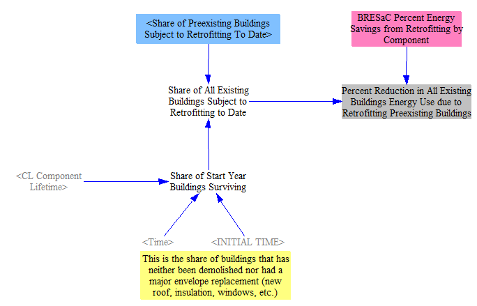
Retrofitting Calculations

The retrofitting policy applies only to preexisting buildings. We first determine the share of buildings that existed in the model start year that are surviving in each year of the model run, using the average building lifetime. We then apply the user's selected policy setting for Share of Preexisting Buildings Subject to Retrofitting to Date to the share of surviving buildings. Finally, we apply a percentage reduction in energy consumption by component for a typical retrofit to the share of existing buildings subject to retrofitting. In the U.S., retrofits are set to reduce energy consumption for the heating and cooling end uses.

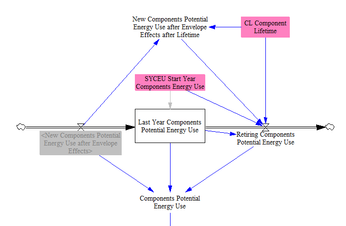
Finding Components Energy Use

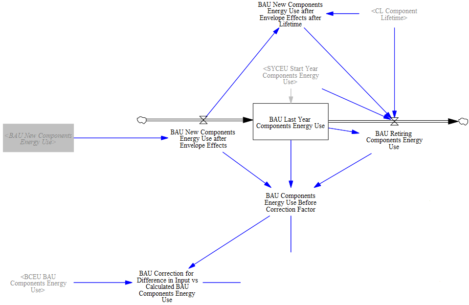
After accounting for policy effects for newly sold components and applying the envelope modifier, we track the potential energy use for the entire stock of building components. We will add in the retrofitting effects later in the calculation flow. We add the energy use for newly sold components to last year's energy use, subtracting out the energy use from retiring components (calculated using the average lifetime of each building component). The relevant structure is shown below:

We next consider building occupants' behavioral responses to higher or lower energy prices. We first determine the change in cost of the fuel that would be needed to run all components at "potential" - that is, before the influence of behavioral response to prices. (This refers to changes in how buildings and appliances are used, not changes in what products are purchased. Price-based changes in what products are purchased are handled by a different section of this page, discussed above.) This is challenging, because the component electrification policy shifted a certain amount of energy use between fuel types (and our elasticities for building service demand with respect to energy cost are disaggregated by fuel type). If we simply compare the BAU and policy cases when the component electrification policy is enabled, it would appear that more electricity was required and less other fuels were required to provide the same services, when what actually happened is that the quantity of services provided by components that use each fuel type has changed.

Accordingly, we construct a "Hypothetical BAU" case that considers what the energy use of components would have been in the BAU case if only the component electrification policy were to act upon that case. First, we apply the electrification policy to the BAU New Components Energy Use, as shown in the following screenshot:

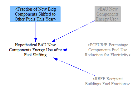
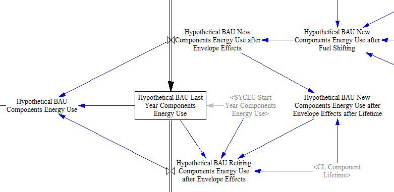
Next, we apply envelope effects, and then we track the hypothetical energy use for the entire building stock in a manner analogous to that which we did for the Policy case, as shown in the following screenshot:

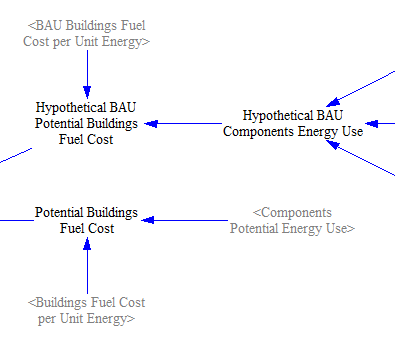
We multiply the hypothetical energy use by the BAU cost of fuels in the buildings sector (by fuel) to get the amount spent on fuels in the hypothetical BAU case. We also calculate the amount spent on fuels in the policy case by multiplying the fuel use in the policy case by the fuel costs in the buildings sector in the policy case. The following screenshot shows this portion of the model:

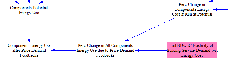
We find the percentage change in fuel cost between these two cases. Then we combine the percent change in energy cost of operating components with an "Elasticity of Building Service Demand wrt Energy Cost" to obtain a percentage change in energy use by building components due to price-demand feedbacks. This is different from the similar elasticity above, which applied only to new components, because that elasticity affects which types of components were purchased and installed. This elasticity affects all components (not just new components), and effects are recalculated each year based on energy cost per unit area -- you do not "lock in" lower or higher energy use for the lifetime of a component that was just purchased. See the next screenshot for the relevant structure:

Next, we subtract the reduction in energy use due to retrofitting (calculated above) from the components energy use.

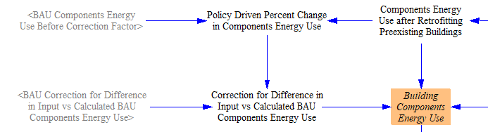
After the adjustments above, we have to apply a correction factor to account for the fact that input data in bldgs/BCEU may not be perfectly in sync with input component lifetime data in bldgs/CL. We find the correction factor within Vensim based on the values in BCEU compared to the calculated BAU version of energy use for building stock, as shown below:

We also apply the correction factor to the policy driven percent change in components energy use, then adjust total energy use for the calculated policy-driven and BAU corrections.

Finally, we adjust energy use for the 'Exogenous GDP Adjustment,' which is no longer used in the U.S. model. This feature can be used to adjust energy and service demand for the COVID-19 induced recession or other economic shocks that are not reflected in collected input data. Because the U.S. EPS input data already reflects COVID-19, we no longer rely on this feature. However, it is still in use in certain international EPS models. This adjustment is applied only after the correction factor to avoid interfering with the correction factor calculations.

Distributed Solar PV Calculations

The model factors in the amount of distributed electricity generation capacity from a variety of sources on-site at buildings. The vast majority of this generation comes from solar PV panels. It also includes four policies that allow the user to increase the amount of distributed solar PV capacity beyond the BAU case.

First, we read in data on the projected BAU capacity of distributed generation sources over the model run. We calculate the increase in distributed capacity in the BAU by looking at the year-over-year change from inputs. We assume retirements of distributed capacity are not significant during the model run timeframe, as they are dominated by solar, which consists mostly of relatively recent equipment. We also include input data on the maximum distributed solar capacity in the region as a validation check on inputs and calculations to prevent downstream errors. The following screenshot shows this structure:

The first policy that can impact distributed generation is a boolean that, if turned on, causes the model to read in a non-BAU projection of distributed generation capacity. This enables the user to easily implement projections from other sources. The second policy to influence distributed generation is a subsidy for distributed solar. The model calculates the effect such a subsidy using an elasticity of distributed solar deployment with respect to subsidy price, which modifies the BAU increase in distributed solar capacity. The additional subsidy lever represents the percentage of distributed solar costs that are not subsidized in the BAU, hence the inclusion of the BAU percent subsidy variable here.

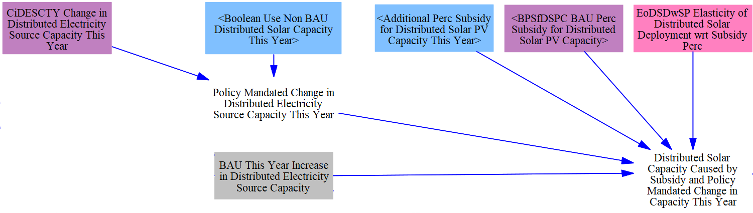
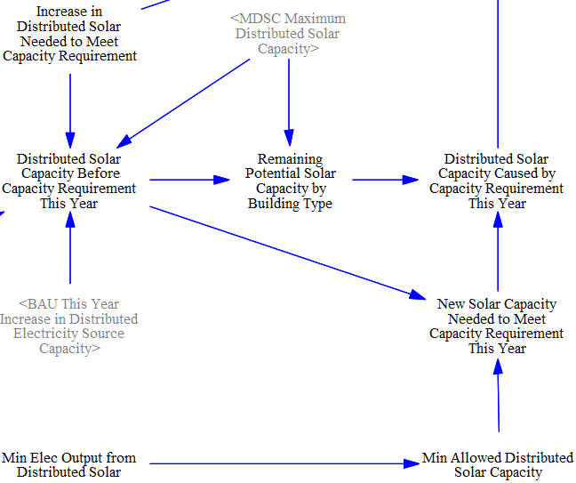
The third policy that can impact distributed generation is a policy specifying a minimum cumulative installed capacity to exist in a given year. For example, this policy could reflect a region's binding target of X GW of rooftop solar be installed by 2030. The increase in new installations needed to meet the capacity requirement is added to the prior year's total installed capacity to determine the total capacity required.

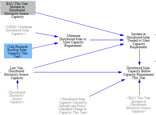
The total installations required to meet the capacity requirement in the last step are used to deteremine how much additional solar, if any, is required this year by the fourth and final distributed generation policy: a carve-out policy requiring a minimum share of all electricity generation to come from distributed solar in a year.

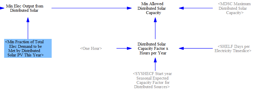
To calculate the effects of the distributed solar carve-out policy, we multiply the total electricity demand (with a one-year delay to avoid circularity) by the minimum allowable fraction of electricity to come from distributed solar PV to find the quantity of distributed solar PV output we require in the current year.

We convert this minimum output to capacity using rooftop solar capacity factors for each electricity timeslice.

The distributed solar installations required by the capacity minimum are subtracted from the installations required by the carve-out, yielding any incremental builds required to meet the carve out.

Finally, we compare the builds required under each of the three cases.

First, if the non-BAU distributed solar capacity boolean is turned on, the model ignores the capacity minimum and carve-out policies' effects. We do this because if the user is using exogenous capacity projections, these policies are likely superfluous and can cause confusion around results.

Second, if the non-BAU distributed solar capacity boolean is turned off, the model compares the new installations driven by the BAU and any subsidies vs. the new installations needed to meet the capacity requirement and carve out. This makes the subsidy policy non-additive to the other two, as a subsidy would more often be used to make a solar mandate affordable for consumers rather than to surpass the ambition of the target itself.

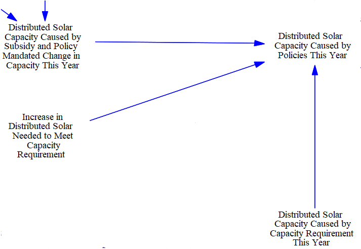
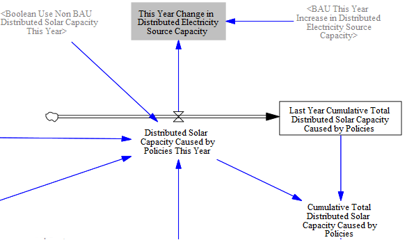
The model then calculates a cumulative total amount of distributed generation deployed due to policies.

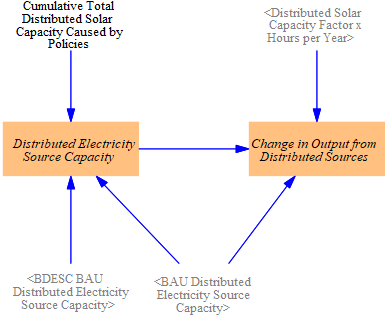
We sum the total capacity in the BAU case with the distributed solar PV capacity caused by policies to find the total distributed capacity (of each power source) in the policy case. We subtract out the BAU electricity source capacity (of each source) and multiply by the distributed source capacity factor to convert the change in capacity to a change in output. Note that although these calculations could be simpler if we only wanted to obtain the change in output from distributed solar, we use the variables "Distributed Electricity Source Capacity" and "Change in Output from Distributed Sources" as outputs (e.g. on the "Web Application Support Variables" tab) and as inputs on the "Electricty Supply - Main" tab, so we need to calculate them explicitly, as shown below:

Outputs

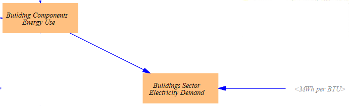
To get total electricity demand from the Buildings sector, we separate out electricity from other fuels and convert the units to MWh.

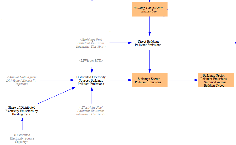
Lastly, we find the total energy use of non-electricity fuels in the Buildings Sector. We multiply the energy use for building components by the emissions indices for each pollutant and for each fuel type, to obtain the direct pollutant emissions from the buildings sector. We also sum emissions across building types in a separate output variable, for ease of reporting total pollutants from this sector, when this is desired by the user. These steps are shown in the following screenshot:

---

This page was last updated in version 4.0.4.