Transportation Sector (cash flow)
The "Transportation - Cash Flow" sheet calculates the changes in amount spent and received for transportation fuels and for vehicles. Changes in price per unit fuel/vehicle and in quantity demanded are both taken into account.
Change in Fuel Spending
The following screenshot shows the model structure used to calculate change in amount spent on fuel, including amount spent on fuel taxes:
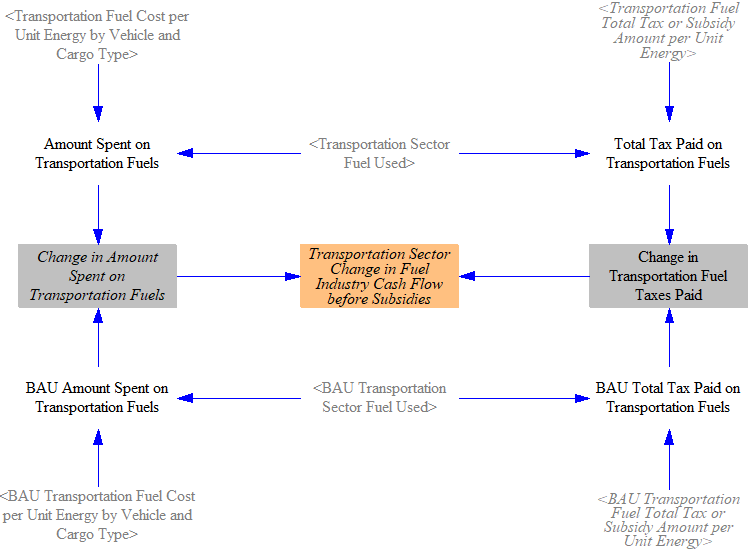
Transportation fuel use by fuel type is multiplied by the fuel cost per unit energy (calculated on the Fuels page) to obtain the amount of money spent on transportation fuels. This value is inclusive of tax. Fuel cost per unit energy is differentiated by vehicle type and cargo type so that the cost of electricity reflects the public/private charging mix specific to each vehicle (see the main transportation page for details). We also multiply the quantity of fuel used by the amount of tax paid per unit energy to find the taxes paid on transportation fuels. These steps are done both for the BAU and the policy cases.
We find the difference in the amount spent on fuel taxes, and we find the difference in the amount spent on fuels. We subtract out the difference in taxes to find the cash flow change for the fuel industry (which is subscripted by fuel type). That is, a reduction in fuel spending is a negative cash flow for the fuel industry, while an increase in fuel spending is a positive cash flow for the fuel industry.
Change in Spending on Vehicles
Policy-related change in spending on vehicles includes several components, including capital and operation and maintenance costs.
Change in Vehicle Costs
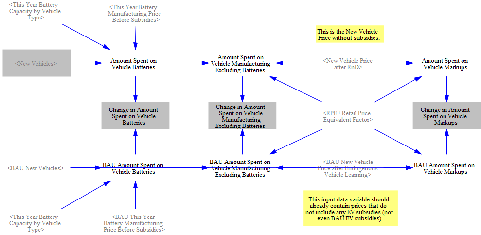
We calculate the number of newly sold vehicles, vehicle prices (before subsidies), and battery prices on the Transportation Sector (main) page. We then multiply these values in both the policy and the BAU cases to find the total amount spent on batteries and non-battery manufacturing. The difference in the amount spent between the two cases reflects the policy-driven change in vehicle spending. This is meant to reflect the total change in cash flow due to vehicle purchases, not the price ultimately paid by the consumer that may be lower due to government subsidies. As the revenues from each component is fed to different sectors, we also break out the amount spent on vehicle markups. Generally speaking, battery spending is fed to the electrical equipment sector, vehicle markups go to auto manufacturers, and the remainder are spread across various industries.
Change in EV Subsidy Payments
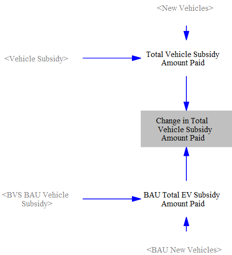
We separately calculate the change in EV subsidies by multiplying the subsidy values and number of vehicles sold in both the policy and BAU cases in order to find the change in total EV subsidies paid.
Change in Vehicle Battery Subsidy Payments
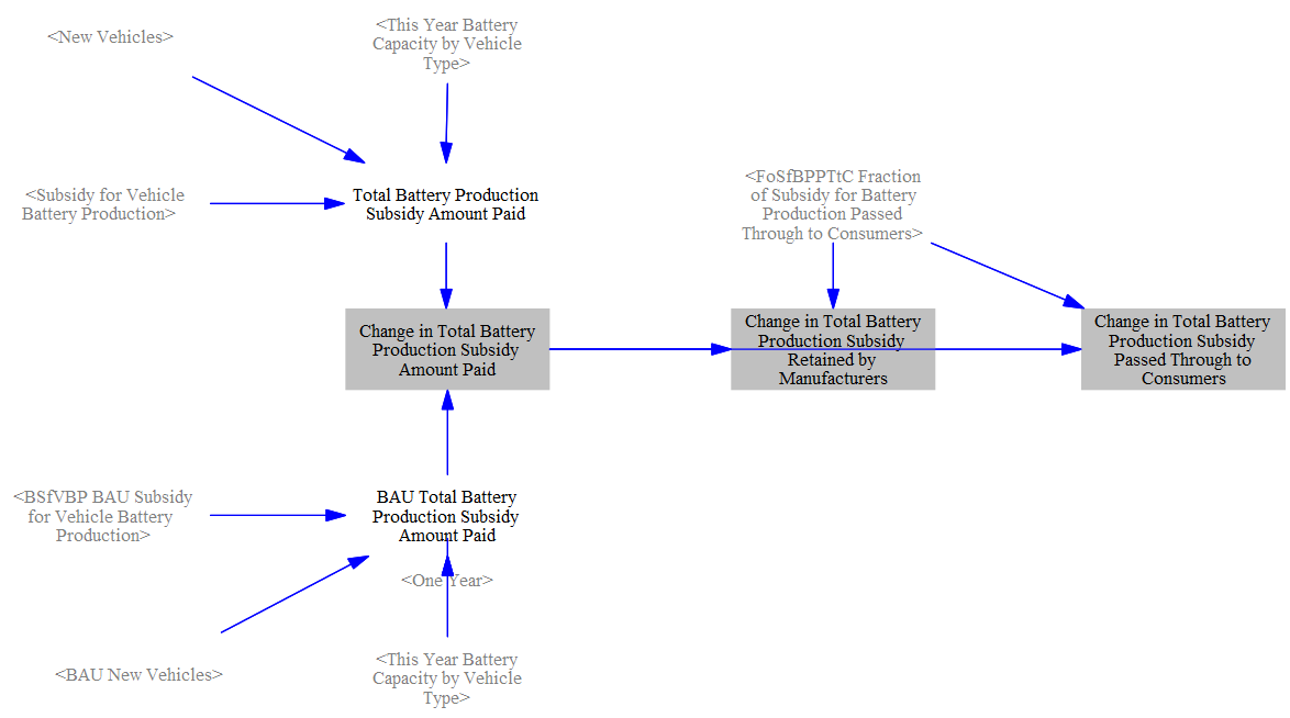
Similarly, we multiply the battery subsidy values by the number of vehicles sold and the battery capacity of each vehicle in both the policy and BAU cases in order to find the change in total subsidies paid. Battery prices and the resulting subsidy pass-through to consumers are tracked by vehicle type, reflecting that battery pack prices vary by vehicle and cargo mode (see the Battery Pack Price Multiplier discussion on the main transportation page). The share of the subsidy passed through to consumers is broken out for revenue tracking purposes.
Change in Other Transportation Costs
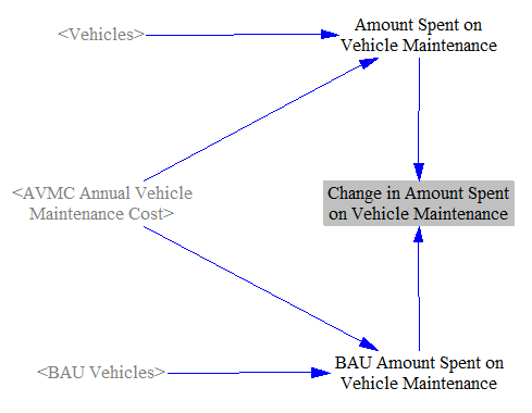
We also calculate the change in the following costs for vehicles: vehicle maintenance, insurance, parking, and licensing/registration/property taxes. These sections find the corresponding costs in both the policy and BAU cases by multiplying cost per vehicle by the number of vehicles in the fleet (not the number of newly sold vehicles, as these costs occur every year of the model run). For example, see the screenshot for the change in vehicle maintenance costs below:
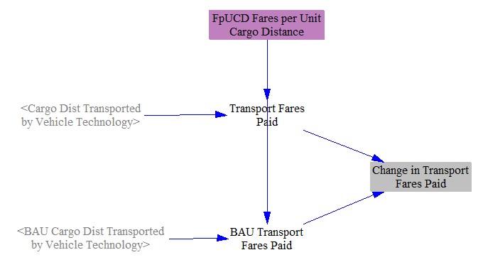
We also calculate the change in transport fares paid. We take input data on fares per unit cargo distance and multiply by the cargo distance transported in both the policy and BAU cases.
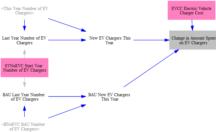
Finally, we calculate the change in amount spent on EV chargers. We take input data on the cost of EV chargers and multiply by the number of chargers deployed in both the policy and BAU cases. This calculation captures the public-charger network funded by the EV Charger Deployment policy. Note that this is distinct from the home-charger installation cost paid by individual passenger LDV BEV buyers, which is included in vehicle pricing on the main transportation page rather than tracked here.
Allocating Changes in Expenditures and Revenue
Changes in Expenditures
Now that we have calculated the changes in spending for the transportation sector, we need to assign those costs to the corresponding cash flow entities, as well as their corresponding ISIC codes (to be used in the Input-Output Model).
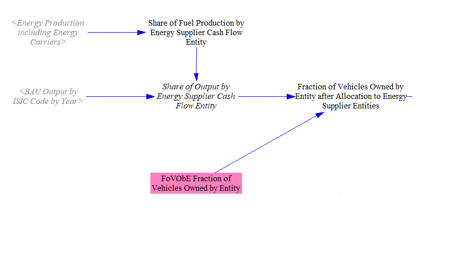
First, we allocate transportation expenditures. To do this, we find the fraction of vehicles owned by each cash flow entity. For most vehicles, the fraction owned by entity is read in as input data. However, we adjust the fraction of freight road vehicles owned by industry based on industrial output, because the share of output provided by the cash flow entities that serve as energy suppliers may vary due to policy.
We then allocate energy expenditures to each of the cash flow entities by multiplying the change in amount spent on transportation fuels by vehicle type by the fraction of vehicles owned by each entity. The model also tracks the change in energy expenditures broken out simultaneously by entity and by fuel type, so downstream calculations can attribute (for example) gasoline-related cash flow effects to consumers separately from electricity-related effects to the same entity.
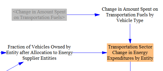
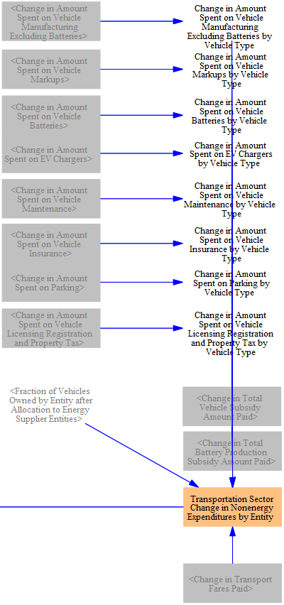
We next allocate nonenergy expenditures. Generally, the categories of spending shown in the screenshot below are assigned to entities based on the change in amount multiplied by the fraction of vehicles owned by that entity. The exceptions are the change in EV and battery production subsidies paid, which are paid wholly by the government, and changes in transport fares (passenger fares are assigned to labor and consumers, while freight fares are assigned to nonenergy industries).
Finally, we use the calculated expenditures by entity variables to also assign expenditures by ISIC code, using data on the percent of output by each ISIC code from the Input-Output Model. We only need to track the transportation sector's changes in expenditures by ISIC code for nonenergy industries, as the EPS separately tracks changes in energy industries.
Changes in Revenue
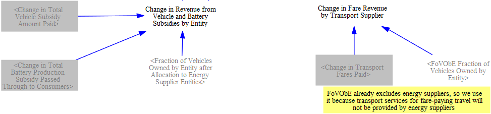
We also need to track which entities and ISIC codes receive money based on transportation sector expenditures. First, we find the change in revenue from EV and battery production subsidies by entity (using the change in subsidies paid and the fraction of vehicles owned by entity). We similarly find the change in fare revenue by transport supplier based on the change in transport fares paid and the fraction of vehicles owned by entity.
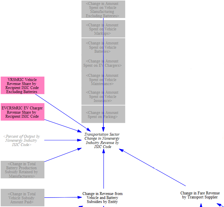
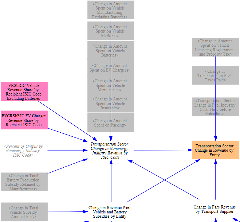
As with expenditures, we want to find the change in revenue by ISIC code for nonenergy industries only. We do this by mapping various categories of expenditures onto the most relevant ISIC code. For example, the amount spent on road vehicles is assigned to the ISIC code for the "motor vehicles, trailers, and semi-trailers" industry, and the amount spent on nonroad vehicles is assigned to the ISIC code for "other transportation equipment" industry. The change in revenue from subsidies for the nonenergy industries entity is assigned based on the percent of output provided by each ISIC code. The change in fare revenue for nonenergy industries is assigned to the ISIC code for "transportation and storage."
Lastly, we also calculate the total transportation sector change in revenue by entity. For the nonenergy industry, this is equal to the sum of the "Transportation Sector Change in Nonenergy Industry Revenue by ISIC Code" variable calculated above. Additional categories of expenditures not included in the nonenergy industries entity are mapped onto the most relevant entities, for example the revenue from vehicle licensing, registration, and property taxes is assigned to the government entity. We also add in the previously calculated change in revenue from subsidies and transport fares.
This page was last updated in version 4.0.5.