Buildings Sector (cash flow)
Change in Fuel Costs and Taxes
The following structure is used to calculate the change in amount spent on fuels, as well as how much of that change goes to fuel suppliers and how much goes to the government (as taxes):
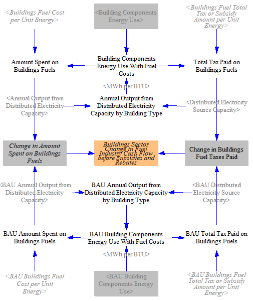
The total amount spent on fuels is calculated by multiplying the energy use by building components (summed across components and disaggregated by fuel) by the fuel cost per unit energy (for each fuel). For electricity specifically, we first net out the annual output from on-site distributed electricity sources (rooftop solar PV, on-site wind) by building type, since households and businesses do not pay the utility for power they generate themselves. The result is the "Building Components Energy Use With Fuel Costs," which represents the energy whose fuel cost actually flows to fuel suppliers. A similar calculation is performed to find the BAU equivalent. The amount of this total that consists of taxes is determined by multiplying the quantity of energy used by the amount of fuel tax per unit energy. Taking the difference between the policy and BAU values for taxes paid gives the change in fuel taxes paid in the buildings sector. Taking the difference between the total amount spent on fuels in the BAU and policy cases gives the change in total amount spent on fuels. We subtract out the difference in taxes to obtain the change in payments to the fuel industry (this is disaggregated by fuel, so the "fuel industry" impacts can be recategorized into more meaningful industry categories on the Cross-Sector Totals page).
Change in Building Component Costs and Taxes
In calculating the effect of policies on building component costs, we only consider components of the types tracked in the Energy Policy Simulator (EPS): heating systems, cooling and ventilation, envelope, lighting, appliances, and other energy-using components. Certain policies, such as the carbon tax, may have a small effect on other components (say, cabinets or countertops) and on the cost of construction activities, but these impacts are not tracked by the model.
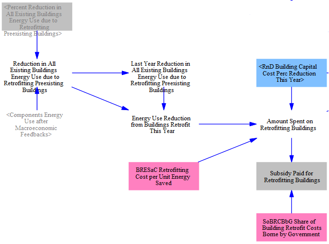
The amount spent on building components in each year of the model run in the BAU case is taken in as input data. We first adjust this amount upward based on the accelerated retrofitting policy, which causes components to be bought more frequently than in the BAU case. We calculate the energy use reduction from buildings retrofitting and multiply it by an assumed cost per unit energy saved from input data. We assume some share of this retrofit cost is borne by government, again defined by input data. Lastly, this amount is reduced by the R&D lever for building capital cost reductions, which lowers the purchase price for new components. The following screenshot shows the relevant structure:
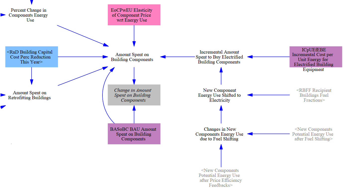
Next, the amount to be spent on BAU plus retrofitted building components is adjusted via three interactions:
- The building component R&D policy can reduce capital costs by a user-specified percentage.
- Various policies (described on the main Buildings Sector page) affect the efficiency of new building components. The percent change in energy use (for the same set of components) is combined with an elasticity of component price with respect to energy use to obtain a change in policy case component costs.
- The fuel use shifting policy changes what type of appliances are purchased by consumers. Typically, this policy represents electrification; e.g., a shift from gas furnaces to heat pumps. Since these components have differing purchase prices, we adjust spending by the incremental amount spent to purchase electrified components, which can be positive or negative depending on the component type.
The following screenshot shows all three interactions and the resulting Amount Spent on Building Components:
Change in Distributed Solar Costs
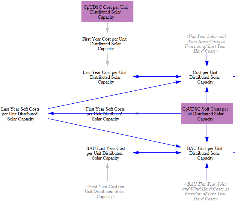
Distributed solar PV costs are handled via the endogenous learning curve for solar PV technology, which is discussed in the Electricity Sector. This means that their costs decline based on total solar PV deployment. We begin with the cost of distributed solar per unit capacity in the start year of the model run and apply the result of the endogenous learning calculation to find the cost per unit capacity in the current year, for both BAU and policy cases.
The same process is applied to the soft costs per unit distributed solar capacity.
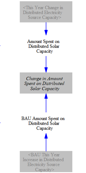
We multiply costs per unit capacity by the amount of distributed solar capacity added in the BAU case and in the policy case to find the total amount spent on distributed solar in the current year in each case. We then take the difference to find the change in amount spent on distributed solar due to policies.
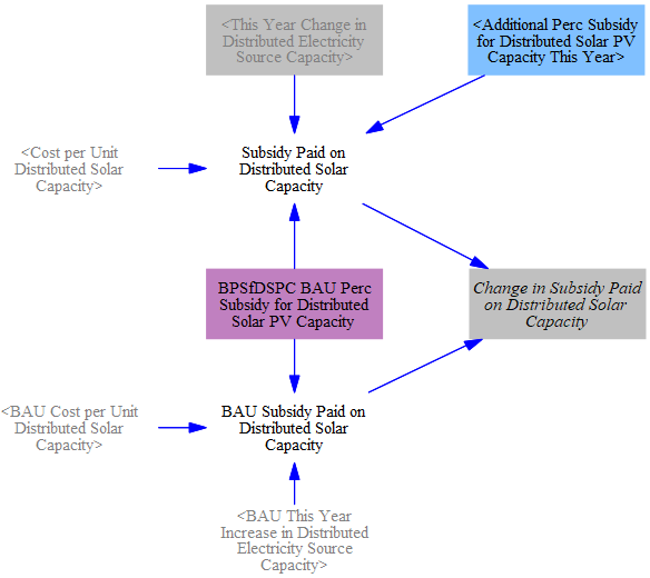
Separately, we calculate the amount spent on subsidies for distributed solar equipment in the BAU and policy cases. We multiply the cost per unit capacity in the BAU and policy scenarios by the year-over-year change in distributed generation capacity and the BAU percentage of costs subsidized (from input data). In the policy case, the percent of the remaining share of capital costs are multiplied in as well.
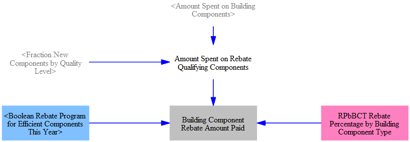
Efficient Component Rebate Payments
To calculate the total amount spent on building component rebates, we first find the total amount spent on rebate-qualifying components. We account for all rebate-qualifying components, not only the ones where the purchase decision was driven by the rebate policy, as "free riders" who would have bought the efficient component also get the rebate. This amount is subsequently multiplied by the percentage of the purchase cost offset by the rebate for all active years.
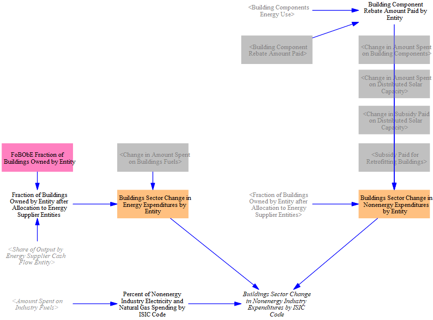
Allocating Changes in Expenditures
Finally, we have to determine which of the model's cash-flow entities (government, industry, and consumers) pay the change in cash flow from fuels and components in the buildings sector. We begin by summing up the change in the amount spent on nonenergy expenses -- such as the building components themselves and various subsidies -- and the change in the amount spent on fuels used in buildings. We divide up these expenditures among cash flow actors by the fraction of buildings owned by each actor. The model also tracks the change in energy expenditures broken out simultaneously by entity and by fuel type, so downstream calculations can attribute (for example) gas-related cash flow effects to consumers separately from electricity-related effects to the same entity. The share of expenses attributed to nonenergy industries is then broken down further into shares paid for by respective ISIC codes (subindustries).
The following screenshot shows the relevant structure:
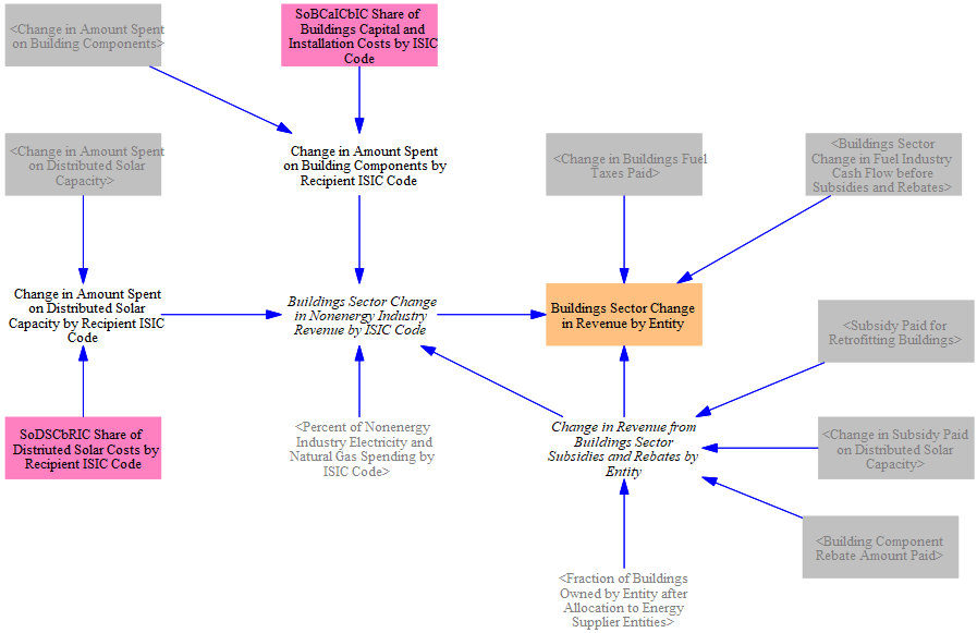
Allocating Changes in Revenue
We also need to determine which of the model's cash-flow entities receive the change in cash flow from fuels and components in the buildings sector. These recipients vary by component type. Data indicating the recipient entity are sourced from inputs. These are segmented by ISIC code, as the portion of non-energy industries' revenue going to labor, taxes, and foreign entities are separated out after the industries' change in revenue is totaled across sectors. Changes in revenue from subsidies and rebates are simultaneously summed across their respective recipients. The calculation flow is shown here:
This page was last updated in version 4.0.5.