Industry & Agriculture Sector (cash flow)

General Notes

The cash flow calculations for the Industry sector are more complicated than the cash flow calculations for any other sector. This is in large part because the Industry sector includes two types of emissions (energy-related emissions and process emissions), with different policies that address each type, as well as requiring the calculation of passthrough costs to consumers. The calculations include the following contributors to the cash flow totals:

• Cash flow impacts of implementing process emissions policies
• Cash flow changes from carbon tax on process emissions
• Cash flow impacts of implementing efficiency and fuel shifting policies
• Cash flow changes from fuel use and taxes affecting fuel
• CCS-related cash flow changes
• Cash flow changes from changes in production
• Passthrough of direct changes in expenditures
• Changes in expenditures due to import substitution
• Carbon tax rebate on exported nonergy products due to carbon border adjustment

Cash Flow Impacts of Implementing Process Emissions Policies

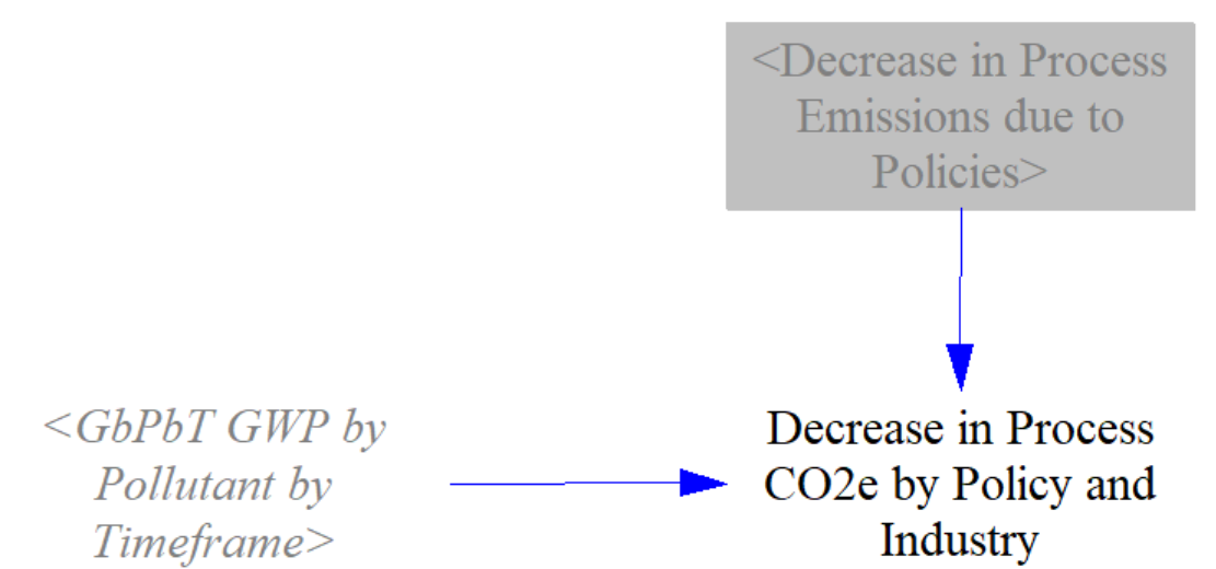
We begin by taking the change in process emissions we found on the Industry and Agriculture - Main sheet and converting it to CO₂e. We use 100-year global warming potential (GWP) values, rather than the user-selected 20-year or 100-year GWP values, because we must use the same timeframe as the EPA source document that provides marginal abatement cost curves, which we use later in the calculation process to convert these changes in CO₂e into changes in cash flow. The following screenshot shows the structure that converts change in process emissions to CO₂e:

Next, we assign all of those emissions reductions to different cost tiers. Our source documents provide marginal abatement curves, which specify a quantity of CO₂e emissions that can be abated at each of a variety of price points (ranging from negative $1150 to -$100 in $50 increments, then up to $100 in $10 increments, and from $100 to $1600 in $50 increments). We assume the lowest-cost abatement opportunities are implemented first. So if the user-specified policy settings cause 10 tons to be abated, the model will assign as many of those tons to the negative $1150 cost tier as possible, then to the negative $1100 cost tier, and so on, until all of the abatement has been assigned to a cost tier. Not all cost tiers will contain abatement potential.

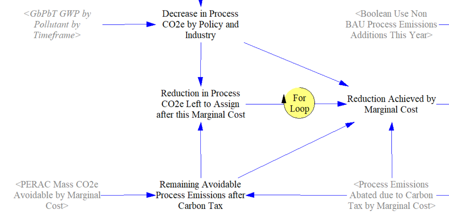
The screenshot below shows how the 'Reduction Achieved by Marginal Cost' is calculated. The calculation is set up to cause Vensim to loop through each element of the "Marginal Abatement Cost" subscript at each timestep. If there are process emissions reductions left to assign at the current Marginal Abatement Cost (meaning all potential in the cheaper Marginal Abatement Cost tiers has been used and there are remaining unassigned reductions), they will be assigned to the current Marginal Abatement Cost, up to the maximum potential in that tier.

This structure also incorporates the variable 'Process Emissions Abated due to Carbon Tax by Marginal Cost,' which was calculated on on the Industry and Agriculture - Main and is already in CO₂e terms. When calculating the remaining emissions reductions to assign, we remove the process emissions abated due to the carbon tax, as those have already been assigned to marginal cost tiers.

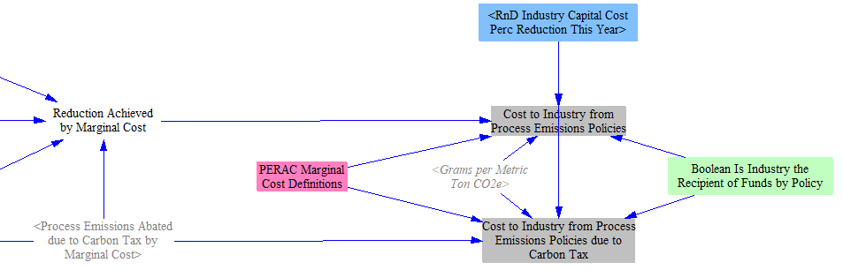
Next, we multiply the number of tons abated at each marginal cost level by the cost definition for that tier. If for a given policy, the funds go to industry (e.g. buying equipment) rather than consumers (e.g. training or hiring workers), we then apply the effects of the user-specified R&D capital cost reduction policy. We do this for process emissions due to the carbon tax separately from other process emissions reductions.

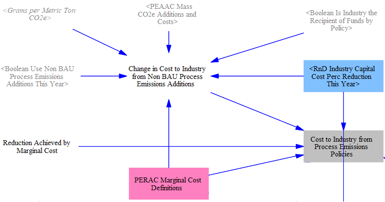
In the process emissions calculations on the Industry and Agriculture - Main sheet, we include a boolean policy to read additional process emissions from input data. We treat these additional emissions similarly to those reduced by other policies, multiplying the number of tons added at each marginal cost level by the cost definition for that tier. These additioanl emissions are fed into the Cost to Industry from Process Emissions Policies.

Cash Flow Impacts of Implementing Efficiency Policies

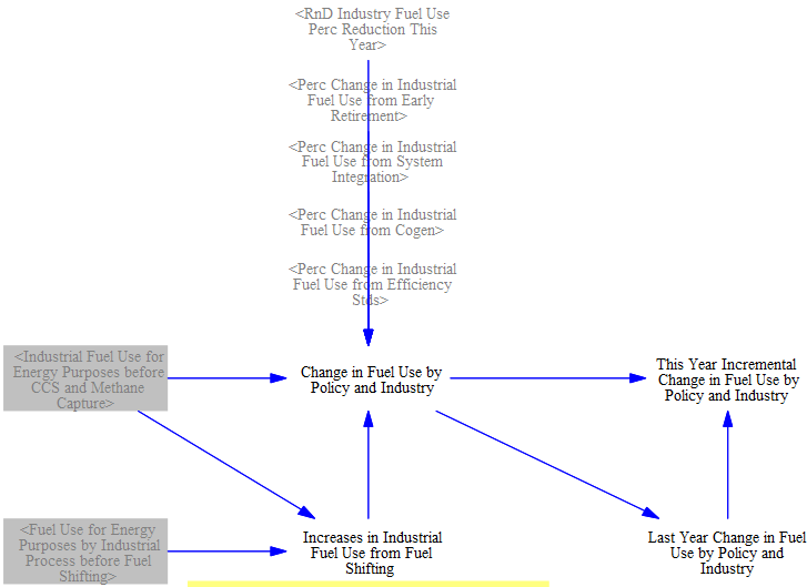
We begin this calculation by determining the additional, incremental change in fuel use (that is, between the policy and BAU cases) in the current year of the model run relative to the prior year. This incremental difference indicates how much additional equipment was needed in the current year, since equipment that enabled fuel savings in past years is still in operation and still provides fuel savings in the current year. For fuel shifting policies, we use increases in industrial fuel use rather than the change in fuel use, since the costs of fuel shifting are based on the purchase of equipment to handle new fuel types. The following structure shows this calculation:

Next, we use input data that provide the cost to implement different efficiency policies per unit of energy saved annually (or, in the case of the fuel switching policy, per unit energy shifted). These factors are multiplied with our incremental fuel savings (from the previous calculation) to determine the current year payments to implement policies (at more stringent levels than the prior year), as shown in the following structure:

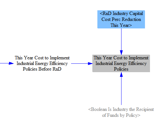
Next, we reduce the cost of equipment purchased due to the policies based on the user's setting for the R&D-driven industrial equipment capital cost reduction policy (by industry category). We only reduce the cost for policies where the main expense for compliance is to buy equipment, rather than to pay workers. The following screenshot shows the relevant structure:

Cash Flow Impacts from Fuel Use and Taxes Affecting Fuel

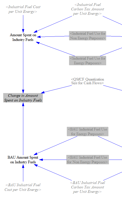
Industrial efficiency policies and changes in production affect the quantity of fuel used, and cross-sector policies such as the carbon tax and fuel taxes can affect the cost per unit fuel. To account for these changes, the fuel used by the Industry sector in the BAU and policy cases (including fuel used to power the CCS process) is multiplied by the fuel cost (disaggregated by fuel) to obtain the total amount spent in each case. We take the difference to find the change in the amount spent. The following screenshot shows the relevant portion of the model:

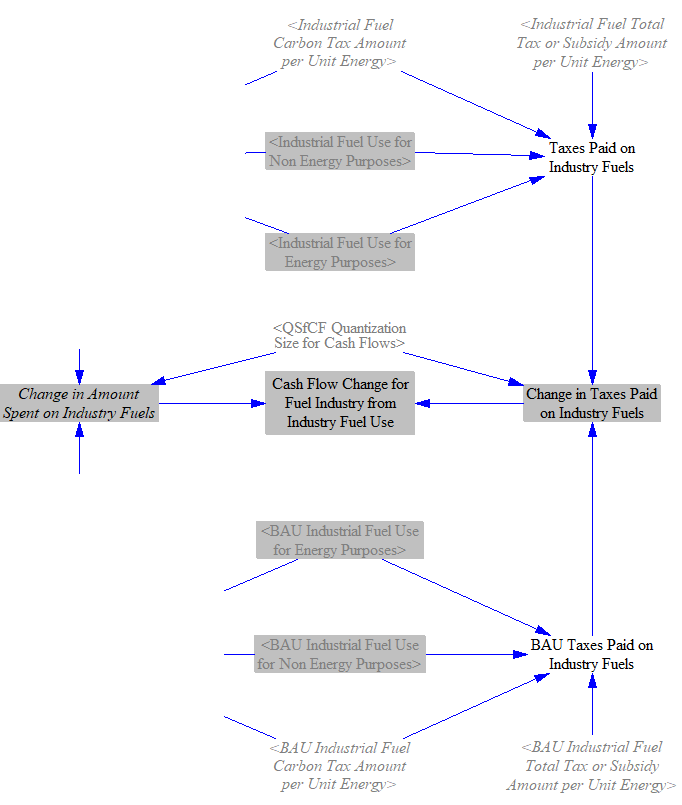
Next, we multiply the amount of fuel consumed for energy purposes in each scenario by amount of fuel tax per unit energy (by fuel) in that scenario to obtain the total taxes paid. However, because carbon tax is only levied on fuels used for energy purposes and not feedstocks, we only apply the carbon tax to 'Industrial Fuel Use for Energy Purposes.' We take the difference in taxes paid between the two scenarios to find the change in taxes paid, and we subtract the change in taxes paid from the change in total fuel spending to find the change in the amount of money going to fuel industries. The following screenshot shows the relevant model structure:

Cash Flow Changes from Carbon Tax on Process Emissions

If the user has set the carbon tax policy to apply to process emissions, process emissions (which were previously untaxed) now incur payments. Additionally, users can select whether the carbon tax applies to non-CO₂ gases, which further determines which process emissions are taxed.

Process emissions are converted to metric tons CO₂e, and the tax rate is applied to determine the amount of carbon tax (by industry category). Note that we use the user-selected GWP timeframe here, under the assumption that when the user sets the carbon tax rate (in $/metric ton CO₂e), they are setting that rate with the chosen GWP timeframe in mind.

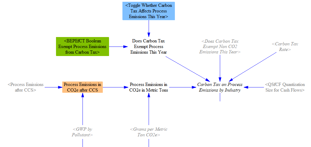
The structure shown above is repeated for the BAU case, and we calculate the 'Change in Carbon Tax on Process Emissions by Industry' as the difference between the BAU and policy cases.

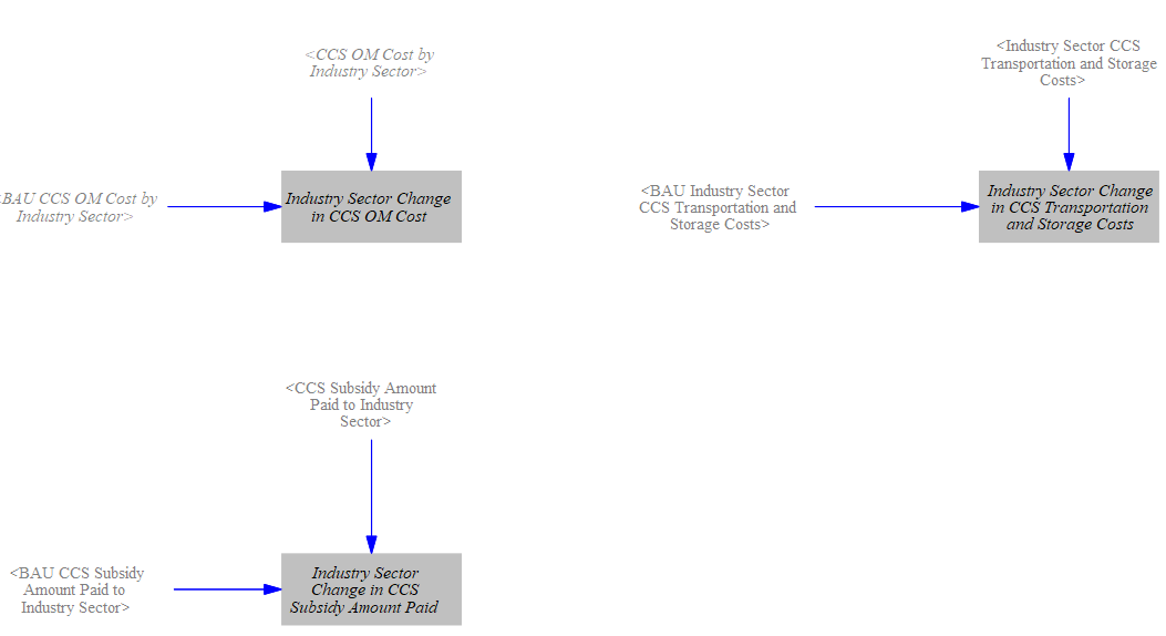
CCS-Related Cash Flow Impacts

The change in Industry sector cash flow related to CCS has three components: differences in CCS capital equipment costs, O&M payments, and carbon tax reductions for sequestered CO₂.

To calculate the change in CCS capital equipment costs, we take the difference in amount spent on CCS capital equipment in the BAU and policy cases. The following screenshot shows the relevant structure:

The change in O&M and transportation and storage costs, as well as the change in CCS subsidies are all handled similarly, as we find the difference in amounts between the BAU and policy cases.

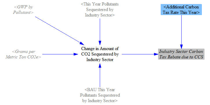
Finally, we take the difference in CO₂ sequestered in the BAU and policy cases, convert from grams of pollutant to grams of CO₂e (which does not change the number, because CO₂ is the only pollutant that can be sequestered, and it has a GWP of 1), and convert to metric tons of CO₂e. This yields the change in CO₂ sequestered by Industry, and we apply the carbon tax rate to find the total tax rebate from CO₂ sequestration. The relevant structure is shown in the following screenshot:

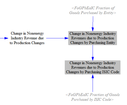
Cash Flow Changes from Changes in Production

Changes in industrial output result in changes in revenue. For each industry category, we adjust BAU output by the percent change in production (note that output is tracked by ISIC code, and we map this onto industry categories here). Because cash flow changes from changes in energy sales are already handled in each demand sector, we exclude the change in cash flow due to changes in energy industry production to avoid double counting. We then add in value-added tax or sales tax, since our input data for output does not inlcude these taxes and we want to reflect the total change in cash flow. This gives us the total change in nonenergy industry revenue due to production changes.

We will need this change in revenue allocated by both purchasing entity and by ISIC code for later cash flow calculations. We do this with input data variables that break down the fraction of goods purchased by entity and by ISIC code. This step is shown below:

Passthrough of Direct Changes in Expenditures

Industries adjust the prices of their goods to reflect policy-driven changes in the amount they must pay to produce those goods, which we define as passthrough costs. Note that we do not pass through changes in expenditures due to changes in production, because an industry that spends less on buying less steel due to producing fewer outputs, for example, can't make its products cheaper due to buying less steel (that is already accounted for in the fact that there are fewer products).

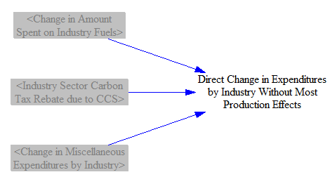
First, we sum up the direct change in expenditures by industry, including the change in fuel spending, any carbon tax rebate, and 'Change in Miscellaneous Expenditures by Industry,' which inlcudes capital and O&M costs calculated elsewhere on this sheet. This gives us the 'Direct Change in Expenditures by Industry Without Most Production Effects.' This variable excludes the effects of production changes on revenue, but it does not exclude every small effect from changes in production. For example, some changes in CCS capital and O&M costs are influenced by changes in production, and the full changes in CCS capital and O&M costs are included in this variable. However, the vast majority of production effects are being excluded.

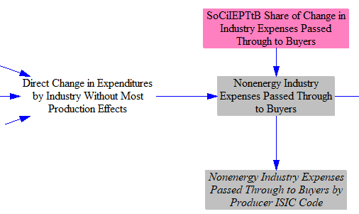
We then find the share of these increased expenditures that is passed through to buyers, which is set through input data. By default, we set this value to 1 to represent full passthrough of changes in expenses to buyers based on the literature. We exclude energy industries because fuel prices are already adjusted by carbon taxes and fuel taxes in each fuel-buying sector. This gives us 'Nonenergy Industry Expenses Passed Through to Buyers,' which is subscripted by industry category. We also create a version of this variable that is subscripted by ISIC code to be used in later calculations.

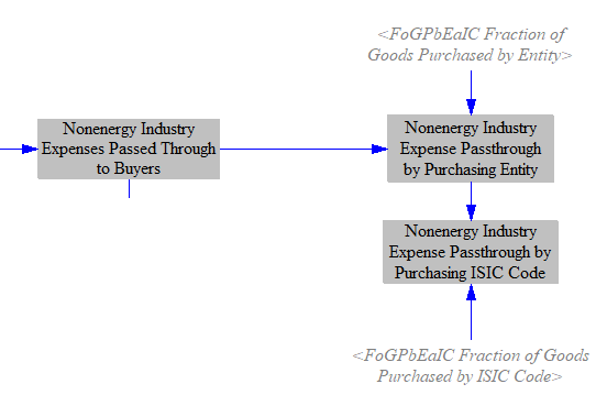
Finally, we need these changes in passthrough costs allocated by both purchasing entity and by purchasing ISIC code for later cash flow calculations. We do this with input data variables that break down the fraction of goods purchased by entity and by ISIC code. This step is shown below:

Changes in Expenditures due to Import Substitution

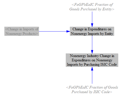
We calculated policy-induced changes in nonenergy imports on the Industry and Agriculture - Main sheet. We need these changes in spending on imports by both purchasing entity and by purchasing ISIC code for later cash flow calculations. We do this with input data variables that break down the fraction of goods purchased by entity and by ISIC code. This step is shown below:

Carbon Tax Rebate on Exported Nonenergy Products due to Carbon Border Adjustment

As shown on the Industry and Agriculture - Main page, the EPS allows for a carbon tax border adjustment for industry products. Users can set whether exported products receive a rebate for the carbon tax when the carbon border adjustment is enabled through a control setting. By default, the rebate for exported products is enabled in the U.S.

To calculate the change in carbon tax rebate for exported nonenergy products, we first need to find the carbon tax per unit industrial output. We calculate this for both the BAU and policy case by finding industrial emissions per unit output (using the total industrial sector CO₂e emissions calculated on the Industry and Agriculture - Main sheet), then multiplying by the carbon tax rate.

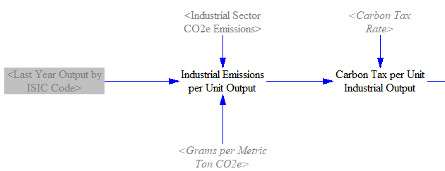
We then evaluate whether the carbon tax border adjustment is enabled. If it is, we check to see whether the rebate for exported products is enabled. If both are enabled, then we apply the 'Carbon Tax per Unit Industrial Output' to the exports of nonenergy products.

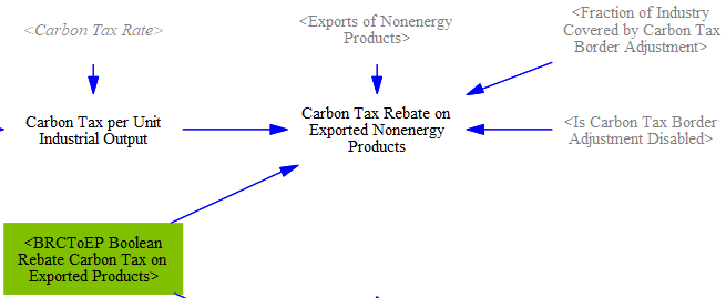
Finally, we take the difference in carbon tax rebated between the BAU and policy cases to find the 'Change in Carbon Tax Rebate on Exported Nonenergy Products.'

Allocating Changes in Cash Flows

Now that we have calculated the changes in spending for the industry sector, we need to sum them to find total expenditures and total revenue, as well as assign those costs to the corresponding cash flow entities and their corresponding ISIC codes (to be used in the Input-Output Model).

Allocating Changes in Expenditures

As covered above, we separately track industry spending on energy and nonenergy products. We therefore separately calculate the total 'Industry Sector Change in Energy Expenditures by Entity' and 'Industry Sector Change in Nonenergy Expenditures by Entity.' We already calculated the change in energy spending above in the variable 'Change in Amount Spent on Industry Fuels,' which is subscripted by industry category. We map the fuel producing industries onto the correct cash flow entities in the step below:

In the screenshot above, we also separate out the 'Industry Sector Change in Energy Expenditures for Natural Gas Production' for use on the Fuels sheet.

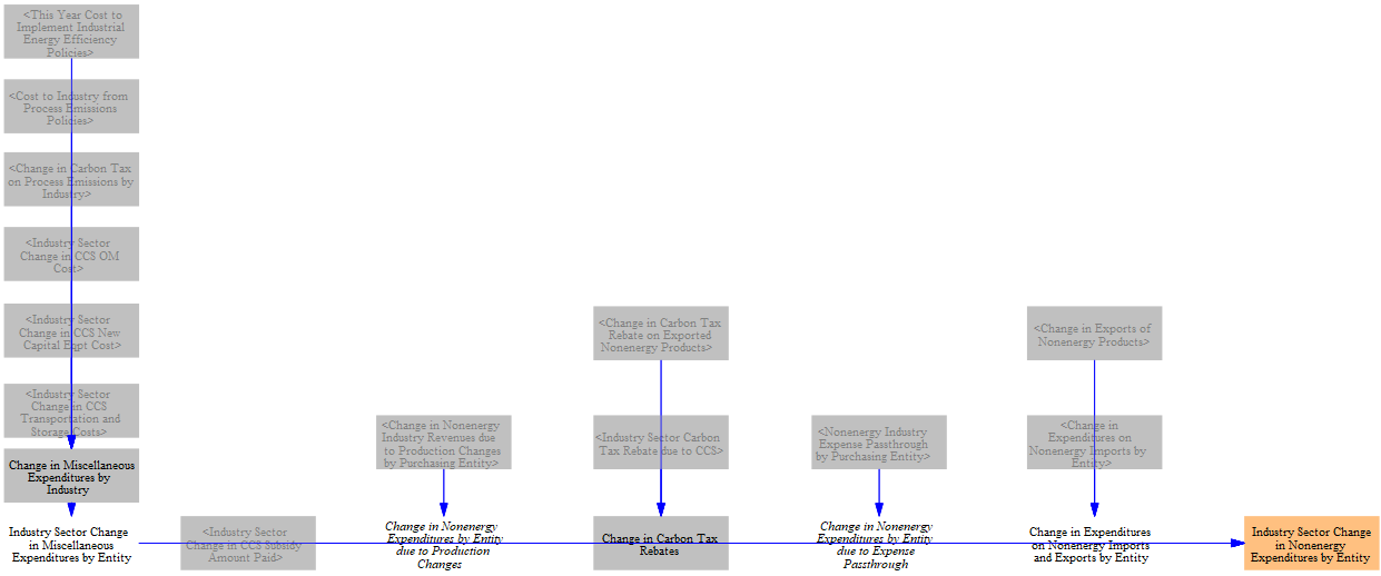
Next, we want to sum up the changes in nonenergy expenditures by entity. We do this in several steps, grouping changes in expenses together by category: 'Change in Expenditures on Nonenergy Imports and Exports by Entity,' 'Change in Nonenergy Expenditures by Entity due to Expense Passthrough,' 'Industry Sector Change in CCS Subsidy Amount Paid,' 'Change in Carbon Tax Rebates,' 'Change in Nonenergy Expenditures by Entity due to Production Changes,' and 'Industry Sector Change in Miscellaneous Expenditures by Entity,' the last of which contains a variety of capital and O&M expenses calculated in the sections above. Where necessary, the structure below maps expenditures that are subscripted by industry category to the relevant cash flow entities. For example, the 'Change in Carbon Tax Rebates' is assigned to the 'government' entity, and expenditures by all nonenergy industry categories are summed together into the 'nonenergy industries' entity.

We also do a similar summation step for nonenergy expenditures by ISIC code, using variables already calculated above. Where expenditures are subscripted by industry category, we map them onto the corresponding ISIC code. This gives us the 'Industry Sector Change in Nonenergy Industry Expenditures by ISIC Code.' Note that this includes cash flow changes to energy suppliers due to changes in their purchases of nonenergy products stemming from overall changes in production of nonenergy products. This is calculated based on purchasing ISIC code, which doesn't separate out the energy suppliers, so we can't assign these cash flows to particular energy suppliers. Therefore, we leave them assigned to the correct energy industry ISIC code.

Allocating Changes in Revenue

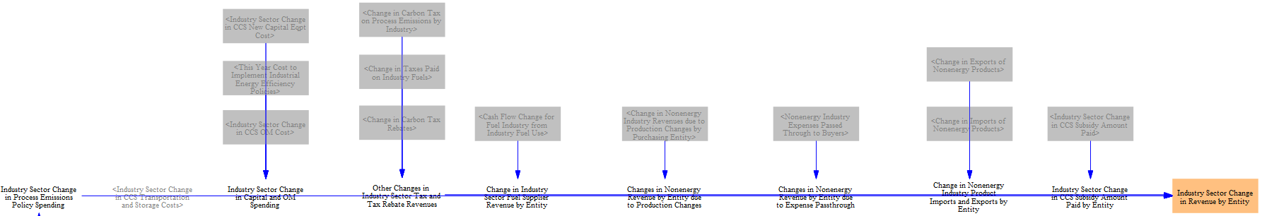
As in the section describing allocating changes in expenditures above, we group changes in revenue together in several categories. Each of the summary variables fed into the final 'Industry Sector Change in Revenue by Entity' shown below have had the industry category subscript mapped to the correct cash flow entities already. Note that the portion of nonenergy industries' revenue going to labor, taxes, and to foreign entities (e.g. if the nonenergy goods were purchased from abroad rather than from a domestic company) are separated out after the change in nonenergy industry revenue has been totaled across all sectors on the Cross-Sector Totals sheet.

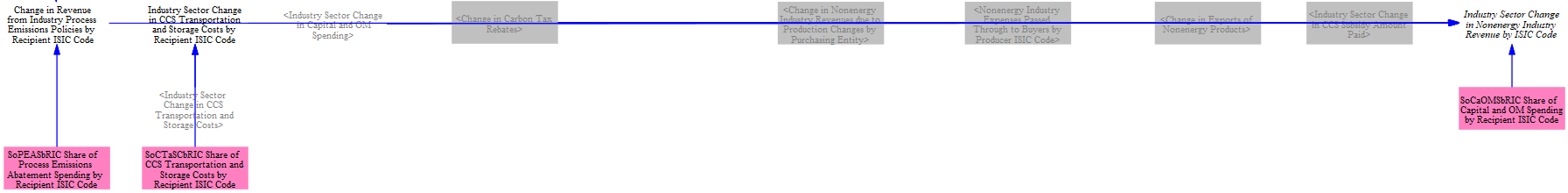
Lastly, we also need the change in nonenergy industry sector revenue by ISIC code to be used in the Input-Output Model. This requires three input data variables that specify 1) the share of process emissions abatement spending by recipient ISIC code; 2) the share of CCS transportation and storage costs by recipient ISIC code; and 3) the share of capital and O&M spending by recipient ISIC code. The corresponding ISIC code for each nonenergy industry category receives revenue from (#1) any carbon tax rebates to the matching industry, (#2a) the matching industry's revenues from selling nonenergy products to any/all cash flow entities, (#2b) any expenses the matching industry passes through in the cost of nonenergy products to buyers, (#3) any revenue from that industry's sales of capital equipment or O&M to other industries, (#4) any revenue from industries' implementation of process emissions policies, (#5) revenue from each industry's change in exports, and (#6) any revenue from each industry's transportation and storage costs.

---

This page was last updated in version 4.0.4.