Comparing Results to Reality or Other Models
We are sometimes asked about the validity of comparing results of the Energy Policy Simulator (EPS) to historical reality, or to outputs from other models, as a means of gauging the accuracy or performance of the EPS. While comparisons with other models may be helpful, comparisons with reality are often problematic. Some considerations to keep in mind regarding these comparisons are provided below.
Comparing EPS Results with Reality
In computer modeling, it is not uncommon for certain types of models to be validated against reality as a means of testing their accuracy. For example, a gridded air quality model may predict the atmospheric concentration of pollutants in each hour of the day for a year in a specific region. If there is an air quality monitor located in that region, the predictions of pollutant concentration from the model may be compared with the hourly data from the air quality monitor. A discrepancy might point to a flaw in the model or its input data files (such as those that specify the meteorology or emissions in that region in each hour).
This type of comparison is generally not useful for evaluating the performance of the EPS. There are a few reasons for this:
Reality is Noisy, and a Close Match Risks Overfitting
Input data sources to the EPS generally forecast gradual changes in energy demand over time, as the input data sources often base their projections on factors that are somewhat predictable over decades, such as population or GDP growth. Where the EPS produces its own baseline projections, such as electric vehicle deployment, these also typically show gradual changes over time, often following linear or S-curve patterns. This reflects the fact that our knowledge of the future over several decades is limited, and we have higher confidence in some of the larger trends (will the population increase in 2045?) than we do in more specific events (will there be a recession in 2045?).
Reality is filled with specific events that are not reasonably predictable by any computer model years in advance. Examples include the timing and magnitude of economic recessions, the results of elections, major court rulings, natural disasters, changes in oil prices, and so forth. These events can have a significant impact on the metrics that the EPS outputs. If the EPS were to be loaded with historical data and then the equations and model structure were tweaked until the EPS could reproduce what actually happened, this would likely worsen the EPS's ability to make accurate future predictions. This counter-intuitive result is due to a statistical phenomenon called overfitting.
Essentially, overfitting occurs when the model simulates not just the underlying trend but also the noise in an input data set. Because noise is random, the ability to simulate historical noise is not helpful in making future predictions. Instead, the best prediction is one that filters out the noise and extrapolates the real trend.
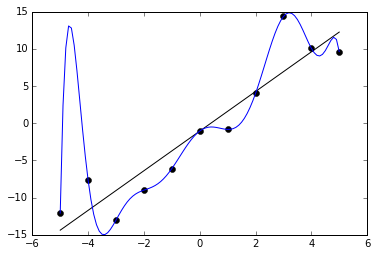
For example, the following graph (from here on Wikimedia Commons, by Ghiles) shows a series of 10 data points and two functions that attempt to fit (explain) the data. The linear model (in black) is a reasonably good but imperfect fit. The tenth-order polynomial model (in blue) fits the data perfectly. However, the linear model is superior, as it is likely to make better predictions when used to extrapolate beyond the ten data points used to create the models.
The strong influence of "noise" (unpredictable events) on historical data, particularly over timespans of just a few years, makes it hard to know whether a closer fit to historical data would be improving or harming the EPS. Various techniques can be used to combat overfitting, such as using a larger quantity (many decades) of historical data, and using only half of the historical data for training the model, then testing the model's predictions on the other half. Unfortunately, these techniques apply poorly to the EPS, as transformative changes in technology, the global economy, and the geopolitical system over the last 50-100 years likely altered many of the underlying trends we wish to capture. Even a good fit with the trends from 1920-1950 wouldn't necessarily say much about the EPS's ability to accurately project outcomes from 2020-2050. This is especially true of developing countries, like China.
History Offers No Counter-Factual Base Case
The main purpose of the EPS is to test the effects of different policies relative to the business-as-usual (BAU) case. But history only happened one way. This means that history provides no guidance as to whether the EPS is correctly simulating the effects of any specific policies or policy packages.
For example, suppose we have a version of the EPS loaded with historical data from five years ago, representing a particular country. During those five years, in reality, that country did not enact any policies not already included in the EPS's BAU case. In the EPS, when we turn on several policies (such as a carbon tax or vehicle fuel economy standards), the EPS estimates the changes in emissions and cash flows that would have resulted from these policies. But since the policies were not, in fact, enacted, history provides no guide as to whether the EPS's estimates of policy impacts would have been accurate.
The same problem occurs if the country did enact non-BAU policies during the last five years. We are able to replicate the country's choices in the EPS, and it predicts the differences the policies would have made relative to BAU. However, history now represents the policy case, not the BAU case, so we again can't tell if the changes projected by the EPS are accurate.
In each of these cases, it is possible to compare certain EPS outputs (those that represent gross quantities, such as emissions) to historical values. But in doing this, one is primarily comparing the EPS model's input data to reality, which does not shed much light on the performance of the EPS model itself.
The EPS has Improved Over Time
One approach to comparing EPS performance with history is to run an older version of the EPS, released years ago, and compare its outputs to what actually happened. (We make past versions of the EPS available on this website.)
However, since its initial release in October 2015, the EPS has undergone numerous improvements, as detailed on the EPS U.S. version history. These improvements include the ability to simulate things that could not be simulated before (such as CCS-equipped power plants), improvements to the way things are simulated (such as hourly electricity demand and dispatch in version 4.0), and numerous bug fixes. Comparing the outputs of a prior version of the EPS to reality would not be an assessment of the performance of the EPS as it exists today, but the performance of an outdated version of the EPS.
It would be possible to take an up-to-date, core version of the EPS and load it with historical data. However, this process would involve a similar amount of labor as adapting the EPS to a new country or region. Given the other challenges noted in this section, it has not, as of yet, been worthwhile to create a version of the EPS with a historical start date for purposes of testing model performance against reality.
Comparing EPS Results with Other Models' Results
While comparing EPS results with reality has serious shortcomings, comparing EPS results with other models' results is often useful, and we routinely do this when adapting the EPS to a new country or region. Like the EPS, other models tend to be forward-looking, and they tend to make smooth projections that omit sources of noise. They sometimes have more than one case (e.g. a base case and several policy cases), so it is frequently possible not only to compare the EPS's BAU case, but also the magnitude of policy effects, between the EPS and another model.
However, there are a couple important points to keep in mind.
It is Better to Understand Differences Relative to Other Models than to Copy Them
No model is perfect, and it is not the goal of the EPS to match any other model precisely. Each model has its own assumptions and methodology to make projections. In some cases, this may be as simple as assuming a linear relationship between passenger vehicle travel demand and population, or between industrial output and GDP. The EPS itself has no view on which demand projections are most likely; the purpose of the EPS is to estimate the effects of policies. Therefore, when comparing the EPS to other models, it is often best to focus first on understanding the reasons for differences between outputs from the EPS and other models. Then, only correct the EPS input data to bring it closer to the other model if you are convinced this would improve projection quality in an absolute sense (not just for the sake of having outputs that are closer to those of the other model).
Sometimes, other models are not transparent, and the only available data are final outputs (such as graphs shown in a publication or government report). Without knowledge of another model's data sources or methodology, it is sometimes not possible to determine the reason for a difference between EPS outputs and that model's outputs. In these cases, the other model's results may suggest an area where a double-check of the EPS data could be helpful, but if no error is found, it often may not make sense to alter EPS data on the basis of this comparison.
Common Causes of Differences in Energy Use or Emissions Relative to Other Inventories or Models
The reported total energy use or emissions in the EPS for various sectors usually differ from those same totals taken from other sources. This is very often a matter of differences in categorization of different emissions types. For example, the EPS considers “waste management” (landfills, water treatment, and wastewater treatment) to be part of the Industry sector. However, the emissions inventory produced by the U.S. Environmental Protection Agency (EPA) considers these facilities to be commercial buildings and hence part of the Buildings sector. The main contribution these facilities make to emissions is via process emissions, rather than energy use. Therefore, for a year covered both by the emissions inventory and by the EPS, emissions from the Buildings sector (particularly methane) are lower in the EPS than in the EPA emissions inventory, and in the Industry sector, they are higher. (The web application interface displays “Waste Management” and “Agriculture” separately from “Industry” to help facilitate comparisons with other models.) In other cases, inventories may omit certain categories of emissions.
Differences in emissions indices are another cause of different emissions results between the EPS and other sources, particularly for non-CO2 gases, because these gases' emissions indices vary more by combustion technology than do CO2 emissions indices. For the United States version of the EPS, we use emissions indices taken from the U.S. Environmental Protection Agency for GHGs and calculate indices for non-GHGs to match data official EPA data.
Different global warming potential (GWP) values also result in different CO2e values. The EPS uses numbers from the IPCC Fifth Assessment Report (released in 2015). Many sources still use older numbers. For example, the 100-year GWP of methane was raised from 25 to 28 in the Fifth Assessment Report, but many sources still use the previous number.
In specific cases, we may choose to use data sources other than official inventories. For example, much of the U.S. input data is sourced from the U.S. Energy Information Administration Annual Energy Outlook (AEO), which uses different methodologies than the EPA for certain sectors.
This page was last updated in version 4.0.4.